Species Distribution Models for invasive species

This article is focused on providing a more in-depth understanding of how Species Distribution Models. If you are interested in a step-by-step guide on how to use the Biosecurity Commons interface for SDM modelling please see our SDM Quick Start Guide.

What is a Species Distribution Model?

A Species Distribution Model (SDM) is a quantitative tool used to estimate the relative suitability of environmental conditions for the establishment and persistence of a particular species across a landscape. For invasive species, SDMs are commonly parameterised using global climatic variables, which are among the most widely available and consistently measured environmental datasets. As a result, they are often referred to as climate suitability models (Camac et al. 2024). By identifying where environmental conditions are likely to support establishment and persistence, SDMs provide an evidence base for a range of biosecurity decisions, including:

• Establishment risk assessment: Identifying regions environmentally suitable for establishment following introduction.
• Surveillance design: Guiding the allocation of surveillance resources towards areas with the highest establishment potential.
• Proof of freedom: Supporting claims of absence by identifying where a species could realistically establish and persist.
• Impact assessment: Delineating the potential extent of establishment to support estimates of economic, environmental, and social impacts.

Types of SDMs

There are two primary approaches to species distribution modelling (Elith 2017; Camac et al. 2024):

Correlative models

Correlative models estimate environmental suitability by identifying statistical relationships between a species' known occurrence records and spatial environmental variables. These relationships are then used to predict the relative suitability of environmental conditions across unsampled locations. Correlative models encompass several broad classes of methods, including discrimination (or two-class) models that contrast species presences with background or absence data (e.g. Maxent, GLMs, GAMs, and boosted regression trees), environmental profile models that characterise the environmental conditions associated with known occurrences (e.g. BIOCLIM and Range bagging), and distance-based approaches that quantify the environmental similarity between candidate locations and the species' observed environmental profile (e.g. CLIMATCH). Correlative models are the most widely used approach in biosecurity because they can be parameterised using readily available occurrence records and globally available environmental datasets. Their primary limitation is that predictions are based on observed associations rather than the biological processes that determine whether a species can survive, grow, reproduce, and persist. Consequently, predictions should be interpreted with caution when extrapolating to novel environments, future climates, or regions that differ substantially from those represented by the occurrence data, as the statistical relationships used to fit the model may no longer hold.

Process-based (mechanistic) models

Process-based (mechanistic) models estimate environmental suitability by explicitly representing the biological, physiological, and demographic processes that determine whether a species can survive, grow, reproduce, and persist under particular environmental conditions. These models encompass a range of approaches, from physiologically based models that explicitly simulate processes such as energy balance, water balance, development, and reproduction (e.g. NicheMapR), to semi-mechanistic models that represent species responses through simplified growth and stress functions informed by experimental or observational data. Because these models are based on the mechanisms that govern a species' response to its environment, they are generally considered better suited to estimating a species' fundamental distribution—that is, the geographic areas where environmental conditions are capable of supporting self-sustaining populations, irrespective of whether the species has dispersed there or whether its realised distribution is constrained by factors such as competition, predation, dispersal limitation, or other biotic interactions. Consequently, they are assumed to be more robust when extrapolating to novel environments or future climates. However, they require detailed experimental or physiological data that are unavailable for most invasive species, making them considerably more time-consuming and difficult to parameterise (Briscoe et al. 2019).

SDMs supported by Biosecurity Commons

Biosecurity Commons currently supports correlative species distribution models (SDMs) that are specifically suited to invasive species applications. In particular, the platform provides integrated support for two profile modelling approaches that estimate a species' environmental niche using occurrence records alone:

• Range Bagging – a presence-only ensemble environmental envelope approach.
• Climatch – a climate similarity approach that compares the environmental conditions at known occurrence locations with those at candidate locations.

Users interested in a broader range of SDM algorithms can instead use our sister platform, EcoCommons, which supports 16 modelling approaches (including Maxent, Generalised Additive Models, Generalised Linear Models, Boosted Regression Trees and others).

Many of the algorithms implemented in EcoCommons are two-class (discrimination) models that distinguish suitable from unsuitable environments by contrasting presence records with absence, pseudo-absence, or background locations. While these methods can perform well in many ecological applications, they require users to make important assumptions about the extent, availability, and distribution of pseudo-absence or background data. These assumptions are often difficult to justify for invasive species, whose realised distributions are typically incomplete because populations are still spreading, have not reached equilibrium, or remain undetected across large parts of their potential range. Consequently, predictions from two-class models can be sensitive to pseudo-absence or background selection, making outputs less robust and less directly comparable across species. For this reason, Biosecurity Commons focuses on profile-based methods that avoid these assumptions and are generally better aligned with the challenges of invasive species risk assessment.

Users wishing to incorporate other SDM algorithms into Biosecurity Commons can do so by first fitting their model in EcoCommons (or locally), exporting the resulting suitability map, and then uploading that output into the relevant Biosecurity Commons workflow (e.g. risk mapping, spread modelling, surveillance design, or impact assessment). This approach allows users to leverage the broader range of modelling algorithms available in EcoCommons while taking advantage of the downstream analytical and decision-support capabilities provided by Biosecurity Commons.

Random Seed

Setting a random seed ensures that the random sampling used by Range Bagging or Climatch is reproducible. Using the same input data, model parameters, and random seed will always produce identical results, making analyses easier to reproduce, validate, compare, and share with collaborators. In most cases, the default seed is appropriate and does not need to be changed unless a different random realisation is specifically required.

Range Bagging

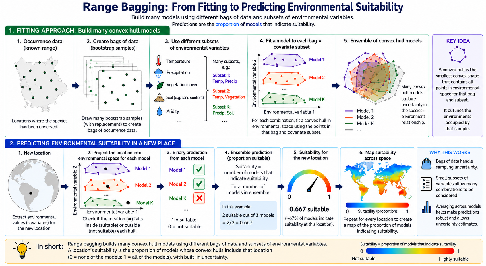
Range bagging (Drake 2015) is a presence-only species distribution modelling approach that estimates the environmental envelope occupied by a species from its known occurrence records. The underlying premise is that locations with environmental conditions similar to those occupied by the species are also likely to be capable of supporting establishment. To estimate this environmental envelope, the method repeatedly fits many simple models using random subsets of occurrence records  and environmental variables. Each model defines the occupied environmental space using a multidimensional boundary (a convex hull), and locations whose environmental conditions fall within this boundary are classified as suitable. The final prediction is obtained by combining the results from all models, with suitability expressed as the proportion of models that classify a location as suitable. This ensemble approach reduces sensitivity to individual occurrence records and predictor variables while providing an intuitive measure of confidence in environmental suitability.

Range bagging is particularly well suited to biosecurity contexts because the primary objective is often to identify where an introduced species could establish if introduced, rather than simply defining its current distribution. By estimating the environmental envelope occupied by a species, the method provides a biologically intuitive estimate of potential establishment risk using only occurrence records. Unlike many other correlative methods, it does not require absence or background data, avoiding several subjective modelling decisions that can substantially influence model predictions.

Range Bagging Parameters

Number of dimensions (Default = 2):
The number of environmental covariates randomly selected for each individual model fit. We recommend retaining the default value of 2, meaning each model is fitted using only two environmental variables. Evidence suggests that ensembles of many simple bivariate models often produce more robust and transferable estimates of environmental suitability than fewer, more complex high-dimensional models. Restricting the dimensionality also reduces the risk of overfitting and allows the ensemble to better account for uncertainty in predictor selection.

Number of models (Default = 1000):
The number of bootstrap models included in the ensemble. Larger numbers improve the stability and precision of suitability estimates by more thoroughly sampling different combinations of occurrence records and environmental covariates. In most applications, 1000 models provides a good balance between computational efficiency and prediction stability, and is sufficient to adequately represent the uncertainty associated with the modelling process.

Proportion of occurrence records sampled for each model (Default = 0.5):
The proportion of occurrence records randomly sampled (with replacement) to construct the convex hull for each model. This parameter controls the degree of variation among ensemble members. There is currently little empirical evidence supporting a universally optimal value because the appropriate proportion depends on the size and quality of the occurrence dataset. A value of 0.5 is generally suitable for large datasets containing hundreds or thousands of records. For smaller datasets (e.g. fewer than 100 occurrence records), higher values are recommended to ensure each bootstrap sample contains sufficient data to estimate a meaningful environmental envelope.

Limit occurrence records (Default = TRUE):
When enabled, each occurrence record can contribute only once to an individual bootstrap sample, even though sampling is performed with replacement. We strongly recommend leaving this option enabled. Doing so reduces the influence of duplicated records within individual models, helps minimise the effects of spatial sampling bias, and produces more representative estimates of the occupied environmental envelope.

Range Bagging Advantages

• Estimates the occupied environmental envelope of a species, making it particularly well suited to identifying areas at risk of establishment during pre-border preparedness, horizon scanning, and early post-border surveillance.
• Does not require absence or pseudo-absence (background) data, avoiding a major source of bias and uncertainty in invasive species modelling.
• Fits large ensembles of simple, low-dimensional models (using small random subsets of environmental variables), an approach that has been shown to reduce overfitting and often provides more robust predictions than fitting a single complex model.
• Explicitly accounts for uncertainty in predictor selection by repeatedly fitting models using different subsets of environmental variables, reducing dependence on any single set of covariates.
• Reduces overfitting and improves generalisation by combining predictions across bootstrap samples of occurrence records and environmental variables, producing robust estimates of environmental suitability that are less sensitive to sampling noise.
• Produces suitability scores that are directly comparable across species, as predictions represent the proportion of ensemble models identifying a location as environmentally suitable.
• Provides intuitive outputs that are easy to interpret, with higher values indicating greater agreement among ensemble models that environmental conditions are suitable.
• Is relatively insensitive to spatial sampling bias compared with discrimination-based approaches because it characterises the occupied environmental envelope rather than contrasting presences against background locations.
• Is computationally efficient and straightforward to parameterise, making it well suited to rapid screening and comparative assessment of large numbers of species.

Range Bagging Limitations

• Restricted to continuous environmental variables because convex hulls cannot readily accommodate categorical predictors.
• Represents environmental limits using broad environmental envelopes and may therefore smooth abrupt ecological thresholds (e.g. frost tolerance or critical temperature limits), potentially overestimating suitability near the edge of a species' environmental niche.
• Assumes that occurrence records adequately characterise the occupied environmental envelope. Sparse or environmentally biased occurrence datasets may therefore underestimate the full range of suitable environmental conditions.
• Like all correlative models, predictions are based on observed environmental associations rather than the biological processes that determine species persistence. Consequently, predictions should be interpreted cautiously when extrapolating to novel environments or future climates.

Climatch

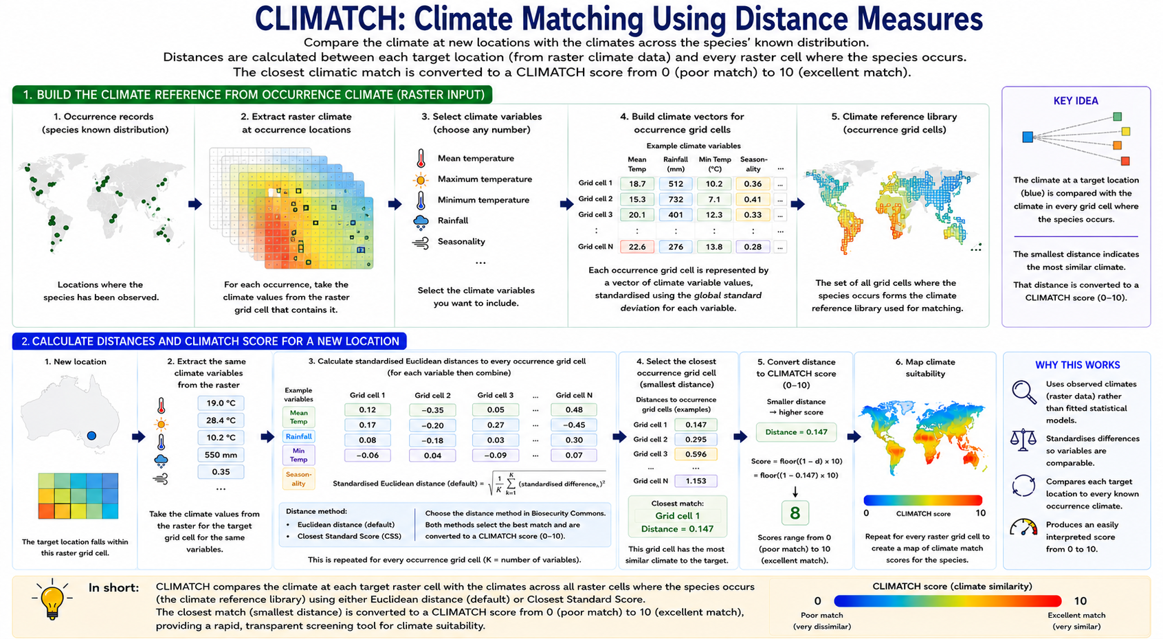
Climatch (Crombie et al. 2008; ABARES 2020) is a climate-matching approach that identifies locations with climatic conditions similar to those observed across a species' known distribution. Rather than fitting a statistical model, Climatch compares the climate at every location in a target landscape with the climates recorded at known occurrence locations. Each climatic variable (e.g. annual rainfall, maximum temperature, or minimum temperature) represents a separate dimension in environmental space, allowing each location to be described by its unique combination of climatic conditions. For every target location, differences in these climatic variables relative to each occurrence location are first standardised to account for differences in scale among variables. Climatic similarity is then calculated using one of two alternative algorithms that combine these standardised differences to produce an overall measure of climatic similarity. 

For each target location, Climatch identifies the occurrence location with the most similar climate according to the selected matching algorithm and assigns a climatic similarity score, with higher values indicating climates that more closely resemble those experienced by the species. Because Climatch relies solely on presence records and direct comparisons of climate, it does not require absence or background data, nor does it involve fitting complex statistical relationships. This makes the method transparent, computationally efficient, and well suited to rapid horizon scanning and preliminary assessments of establishment risk. 

Unlike Range Bagging, which estimates the occupied environmental envelope of a species by identifying the range of environmental conditions associated with known occurrence records, Climatch identifies locations whose climates most closely resemble those already occupied by the species. Climatch therefore measures climatic similarity rather than estimating a species' environmental limits or environmental suitability. Consequently, it is best regarded as a climate analogue method for rapid screening, whereas Range Bagging provides a more robust estimate of environmental suitability and is generally preferred when sufficient occurrence data are available.

CLIMATCH Parameters

Maximum range distance (Default = 50 km)

The maximum distance (km) used to associate each occurrence record with the nearest climate data point (weather station or raster cell). Occurrence records located further than this distance from a valid climate data point are excluded from the analysis. This parameter is primarily intended to accommodate small spatial mismatches between occurrence locations and climate datasets (e.g. differences in coastline position, raster resolution, or coordinate precision).

For most applications, the default value of 50 km is appropriate and should not require modification. Larger values may be appropriate when using coarse-resolution climate datasets or occurrence records with lower spatial accuracy, whereas smaller values may be preferable when working with high-resolution climate data and precisely georeferenced records. 

Climatch algorithm (Default = Euclidean)

The algorithm used to calculate climatic similarity between occurrence locations and the target landscape.

Two algorithms are available:

Euclidean (recommended):
Calculates the standardised Euclidean distance between the climate at each target location and every occurrence location across all selected climatic variables. Climatic differences are averaged across variables to produce an overall measure of climatic similarity, and the occurrence location with the smallest overall distance is used to derive the final Climatch score. Because all climatic variables contribute equally to the final score, this method provides a balanced assessment of overall climatic similarity and is recommended for most biosecurity applications. 

Closest Standard Score (CSS):
Calculates the standardised difference for each climatic variable separately and assigns each difference to one of ten decile classes based on a half-normal distribution. For each occurrence location, the algorithm identifies the worst-matching climatic variable (the highest decile score). The final Climatch score is then based on the occurrence location whose worst-matching climatic variable is least dissimilar to the target location (a "max-then-min" approach). Consequently, climatic similarity is determined by the single climatic variable that differs most between locations, rather than by the average difference across all climatic variables. 

For most biosecurity applications we recommend using the default Euclidean algorithm because it provides a balanced measure of overall climatic similarity. The Closest Standard Score algorithm may be useful when users wish to place greater emphasis on limiting climatic factors or reproduce analyses performed using historical Climatch implementations. 

Logical checkbox: Output as 0–1 instead of 0–10 

By default, Climatch produces climate match scores ranging from 0 (poor climatic match) to 10 (excellent climatic match). Enabling this option linearly rescales the output to a 0–1 range, making it more convenient for use as a relative suitability layer in downstream workflows, such as the abiotic suitability component of the establishment potential workflow. Note that the rescaled values represent relative suitability, not absolute probabilities of establishment.

CLIMATCH Advantages

• Does not require absence or pseudo-absence (background) data, avoiding a major source of bias and uncertainty in invasive species modelling.
• Can be applied when relatively few occurrence records are available, making it useful for newly emerging invasive species where distribution data are sparse.
• Rapidly identifies regions with climates analogous to those occupied by the species, making it well suited to horizon scanning, pre-border preparedness, and preliminary establishment risk assessments.
• Produces climatic similarity scores that are directly comparable across species, facilitating consistent screening and prioritisation of multiple invasive threats.
• Computationally efficient and straightforward to parameterise, requiring only occurrence records and climatic variables.
• Produces transparent and intuitive outputs because predictions are based on direct comparisons of climatic similarity rather than fitted statistical relationships.

CLIMATCH Limitations

• Measures climatic similarity rather than estimating a species' occupied environmental niche or environmental suitability, so outputs should not be interpreted as probabilities of establishment.
• Does not account for uncertainty in predictor selection, as predictions are based on a single user-defined set of climatic variables rather than an ensemble of alternative predictor combinations.
• Does not explicitly model interactions or nonlinear relationships among climatic variables, potentially limiting its ability to represent complex ecological responses.
• Restricted to continuous climatic variables and cannot directly incorporate categorical predictors such as land use or vegetation classes.
• Generally less suitable for fine-scale ecological modelling or estimating environmental limits than methods such as Range Bagging that explicitly characterise a species' occupied environmental envelope.

The importance of filtering & cleaning occurrence records

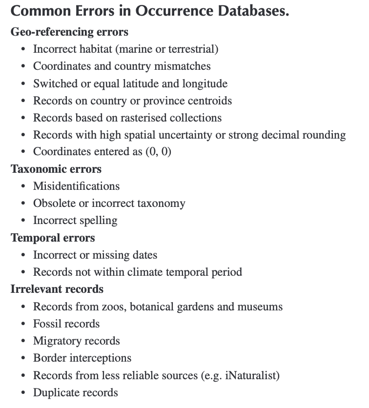
The accuracy of a correlative SDM depends on the quality of input occurrence records. Biosecurity Commons allows users to upload their own occurrence records or use our integrated APIs to pull records from biodiversity databases such as the Global Biodiversity Information Facility (GBIF), Atlas of Living Australia (ALA) or Ocean Biodiversity Information System (OBIS). Occurrence records from online databases like the GBIF often contain errors that can introduce significant bias (Camac et al. 2024).

Importing and filtering occurrence records

When pulling records from such databases, users have multiple options for filtering records. Specifically there are a range of filtering options for improving the quality of occurrence datasets prior to modelling by removing records that are unlikely to represent established populations or that are incompatible with the selected environmental data. Records can be filtered by occurrence status, record type (e.g. observation or preserved specimen), collection date, and geographic location. Users can also exclude records without geographic coordinates and restrict analyses to countries where the species is known to be established, helping to remove transient, introduced, or erroneous records. Cross-referencing occurrence records against authoritative distribution datasets, such as CABI's Invasive Species Compendium, is particularly useful for identifying countries where a species is known to have established populations and excluding records from countries where occurrences are likely to represent interceptions, failed introductions, or other transient observations. Aligning the temporal range of occurrence records with the environmental datasets used for modelling (e.g. post-1970 records when using WorldClim 2.1) is also recommended to improve consistency between species observations and the environmental conditions represented by the predictor variables.

Additional cleaning of records

Biosecurity Commons also provides a suite of automated occurrence-cleaning routines that complement the import filters described above. These routines are based on the R package CoordinateCleaner and are designed to identify and remove common georeferencing errors and artefacts frequently found in biodiversity databases. Eliminating these erroneous records helps improve the quality of occurrence datasets and reduces the likelihood of fitting models to locations that do not represent genuine species occurrences.

The following cleaning routines are available:

• Capital centroids: Removes records located within a user-defined radius (default: 5000m) of national or state capital centroids, which often indicate imprecisely georeferenced records.
• Country centroids: Removes records located within a user-defined radius (default: 5000m) of country centroids, which are commonly assigned when precise collection locations are unavailable.
• Equal coordinates: Removes records where latitude and longitude are identical, a common data-entry error (e.g. 35°, 35°).
• Biodiversity institutions: Removes records located within a user-defined radius (default: 100m) of known biodiversity institutions (e.g. museums, herbaria, universities, botanical gardens), where specimen storage locations may have been mistakenly recorded instead of collection locations.
• GBIF headquarters: Removes records located within one degree of the GBIF headquarters in Copenhagen, Denmark, which are typically artefacts of data processing rather than true species occurrences.
• Zero coordinates: Removes records located at, or within a user-defined radius (0.5 degrees) of the coordinate origin (0°, 0°), a well-known placeholder for missing geographic coordinates.
• Sea locations: Removes terrestrial occurrence records located in marine environments, helping identify records with erroneous coordinates or georeferencing errors.

Importance of expert review (Gold standard)

Filtering and automated cleaning routines are designed to identify common errors and artefacts in biodiversity datasets, but they cannot determine whether an individual occurrence record is biologically plausible. Where feasible, the cleaned dataset should be reviewed by subject-matter experts to identify remaining issues such as misidentified specimens, transient or intercepted records, spatial outliers, coordinate errors, or records from regions where the species is not known to have established populations. Expert review provides an important final quality-assurance step, helping ensure that occurrence records accurately represent the species' occupied distribution before model fitting.

Selecting model covariates

The choice of environmental covariates is one of the most important—and often most challenging—aspects of species distribution modelling (Camac et al. 2024). At broad spatial scales (e.g. continental or global analyses), climate is generally the dominant determinant of species distributions and therefore forms the basis of most biosecurity risk assessments. At finer spatial scales, however, additional environmental factors such as host availability, land use, topography, soils, or vegetation may further influence whether a species can establish and persist.

Biosecurity Commons supports a wide range of environmental datasets, allowing users to tailor predictor variables to the ecology of the species being modelled. Commonly used datasets include:

• WorldClim: The most widely used environmental dataset for species distribution modelling, providing 19 biologically meaningful (BIOCLIM) variables describing long-term patterns in temperature and precipitation (e.g. Annual Mean Temperature, Temperature Seasonality, Annual Precipitation and Precipitation of the Warmest Quarter) at spatial resolutions as fine as approximately 1 km.
• CHELSA: High-resolution climate surfaces that explicitly account for topographic effects and may provide improved estimates of climate in mountainous regions.
• CliMond: Global climate datasets that include historical climate surfaces and future climate projections.
• Climate Research Unit (CRU): Monthly climate datasets that can be useful for generating custom climatic summaries or temporal analyses.
• Non-climatic datasets: Additional predictors such as elevation, terrain derivatives (e.g. slope or aspect), soils, land use, vegetation, or host distributions can be incorporated where these factors are expected to influence establishment or persistence.

Selecting multiple predictor datasets & common resolution

Biosecurity Commons allows users to combine multiple predictor datasets, which may have different spatial resolutions. To ensure all continuous predictors align, datasets are automatically resampled to a common grid. Users can choose whether this common resolution matches the finest (smallest grid cells) or coarsest (largest grid cells) input dataset. Irrespective of method chosen, Biosecurity Commons will utilise  bilinear interpolation to resample predictor inputs to a common resolution/grid.

Selecting predictor variables

Selecting an appropriate set of predictor variables requires careful consideration of both the species' biology and the modelling approach. Although datasets such as WorldClim provide 19 BIOCLIM variables, many describe similar aspects of climate and are therefore highly correlated. Including large numbers of correlated or biologically irrelevant variables may increase model complexity without improving predictive performance and can make model interpretation more difficult. Where possible, predictor variables should be selected a priori based on ecological knowledge of the species, ensuring they represent environmental factors likely to influence survival, growth, reproduction, or persistence.

For most continental-scale biosecurity applications, we recommend using the WorldClim BIOCLIM variables as a starting point because they are widely used, well validated, and facilitate comparison among studies. However, the optimal subset of variables will differ among species and applications, and there is rarely a single objectively "correct" set of predictors.

Importantly, different modelling approaches vary in their sensitivity to predictor selection. Methods that fit a single model(e.g. Climatch or Maxent) require users to carefully select an appropriate set of environmental variables, as predictions depend entirely on that choice. In contrast, Range Bagging explicitly accounts for uncertainty in predictor selection by repeatedly fitting large ensembles of low-dimensional models using random subsets of environmental variables, making predictions less dependent on any single combination of covariates.

Assessing extrapolation and environmental novelty

Species distribution models are generally most reliable when making predictions within the range of environmental conditions represented by the occurrence records used to fit the model. Predictions become increasingly uncertain when projected into environments that differ substantially from those represented in the training data, as the model must extrapolate beyond the environmental conditions on which it was developed. This commonly occurs when projecting models to new geographic regions, future climates, or when occurrence records do not adequately capture the full environmental range occupied by the species.

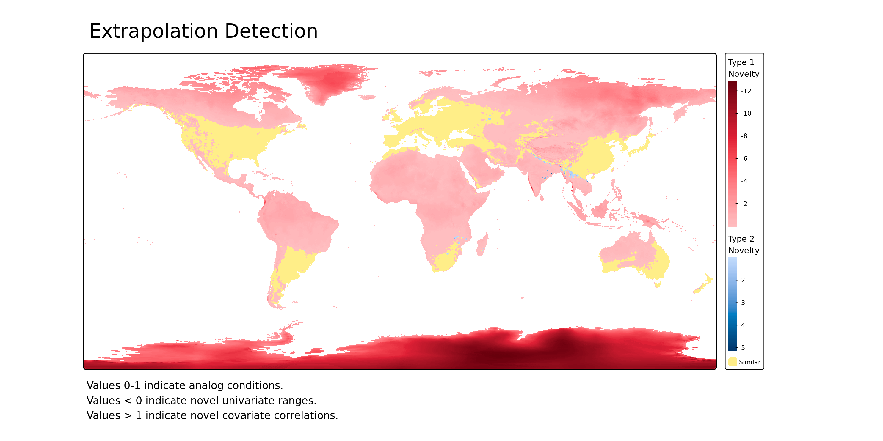
Environmental novelty can arise in two ways. First, one or more environmental variables may fall outside the range observed during model fitting (Type 1 novelty). Second, all environmental variables may individually lie within their observed ranges but occur in combinations that were not represented in the training data (Type 2 novelty). Both forms of novelty reduce confidence that model predictions are supported by observed data and should therefore be considered when interpreting suitability maps.

To help identify areas where extrapolation occurs, Biosecurity Commons provides two complementary diagnostic methods: MESS (Multivariate Environmental Similarity Surface) (Elith et al. 2010) and ExDet (Extrapolation Detection) (Mesgaran et al. 2014). Together, these methods enable users to identify where predictions are supported by environmental conditions represented in the occurrence data, and where they rely on extrapolation into novel environmental space.

MESS (Multivariate Environmental Similarity Surface)

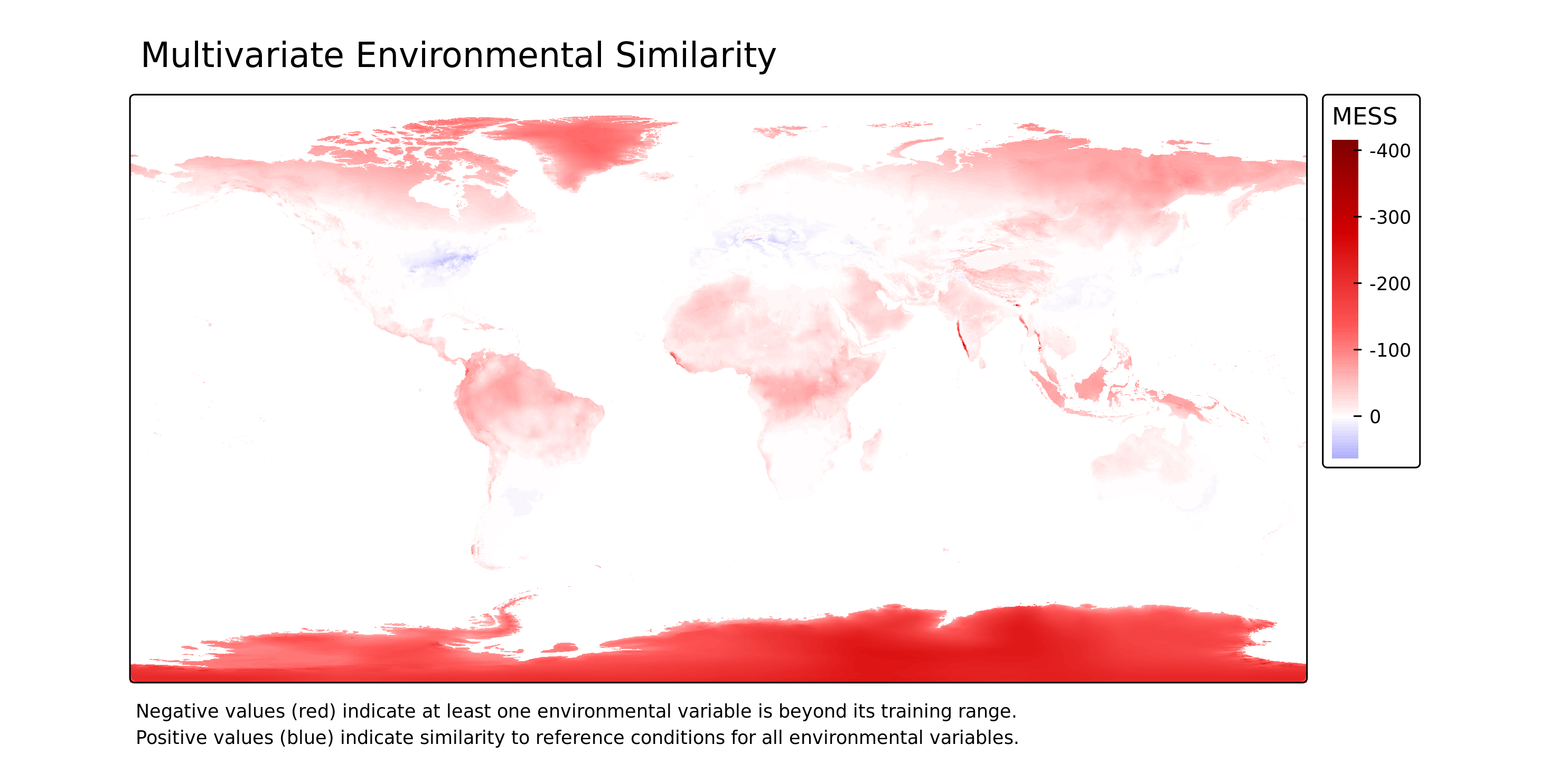
MESS (Elith et al. 2010) quantifies how similar the environmental conditions at each prediction location are to those represented by the occurrence records used to fit the model.

• MESS > 0: All environmental variables fall within the range represented by the training data, indicating predictions are being made within the observed environmental domain.
• MESS < 0: At least one environmental variable falls outside its observed range, indicating extrapolation into novel environmental conditions.

In addition to the MESS similarity map, Biosecurity Commons produces a companion raster identifying the environmental variable contributing most strongly to the MESS score at each location. This helps users identify which environmental variable is primarily responsible for environmental novelty.

ExDet (Extrapolation Detection)

ExDet (Mesgaran et al. 2014) provides a more comprehensive assessment of extrapolation by identifying both the presence and the type of environmental novelty.

• ExDet ≥ 0: Environmental conditions fall within the environmental space represented by the training data.
• ExDet < 0: Environmental conditions exhibit extrapolation into novel environmental space.

Unlike MESS, ExDet distinguishes between two forms of environmental novelty:

• Type 1 novelty (NT1; univariate novelty): One or more environmental variables fall outside the range observed during model fitting.
• Type 2 novelty (NT2; combinatorial novelty): All environmental variables individually fall within their observed ranges, but occur in combinations that were not represented in the training data.

Biosecurity Commons produces an overall ExDet map identifying the dominant form of environmental novelty at each location, together with companion rasters identifying the environmental variable contributing most strongly to Type 1 and Type 2 novelty. These outputs help users determine not only where extrapolation occurs, but also which environmental variables are responsible.

All extrapolation outputs are provided as georeferenced GeoTIFF rasters suitable for further spatial analysis, together with publication-quality PNG images for rapid visual interpretation.

Interpreting extrapolation

Environmental novelty does not necessarily indicate that model predictions are incorrect. Rather, it identifies locations where predictions rely on extrapolation beyond the environmental conditions represented in the occurrence data and should therefore be interpreted with greater caution. Areas exhibiting extensive Type 1 or Type 2 novelty indicate that model predictions are less well supported by the available occurrence data and may warrant additional occurrence records, alternative modelling approaches, or independent validation before being used to support management or policy decisions.

Common Mistakes in SDM

Confusing environmental suitability with establishment risk

Species distribution models estimate the environmental suitability of a location, not the overall likelihood that a species will establish. A location may be highly suitable but have negligible establishment risk if the species is unlikely to arrive, required hosts are absent, or other ecological constraints prevent persistence.

Best practice: Interpret SDM outputs as only one component of establishment risk. Where possible, combine environmental suitability with estimates of arrival likelihood and biotic suitability within an integrated biosecurity risk assessment framework.

Using incomplete or inappropriate occurrence records

Species distribution models should be fitted using occurrence records that represent the full range of environmental conditions occupied by established populations. Restricting analyses to response records, surveillance detections, recent incursions, or a subset of available occurrence records may substantially underestimate the species' occupied environmental niche and lead to overly conservative predictions. Likewise, occurrence datasets may contain transient or intercepted individuals, spatial errors, duplicate records, or misidentified specimens that can bias model predictions.

Best practice: Where possible, use all available occurrence records from established populations across the species' known distribution. Clean occurrence datasets using automated quality-control tools (e.g. CoordinateCleaner), restrict records to countries where the species is known to be established (e.g. using CABI distribution data or expert knowledge), and undertake expert review where feasible before fitting the model.

Selecting inappropriate environmental predictors

The choice of environmental covariates is one of the largest sources of uncertainty in species distribution modelling. Including large numbers of highly correlated or biologically irrelevant variables can reduce model interpretability and, for some modelling approaches, increase the risk of overfitting. Conversely, omitting important environmental drivers may reduce predictive performance.

Best practice: Select predictor variables based on the known biology and ecology of the species rather than data availability alone. Where possible, choose variables that are expected to influence survival, growth, reproduction, or persistence. Consider the implications of predictor uncertainty when interpreting model outputs.

Ignoring extrapolation diagnostics

Species distribution models become increasingly uncertain when projected into environmental conditions that were not represented in the occurrence data used to fit the model. This is particularly common when transferring models to new geographic regions or future climate scenarios.

Best practice: Use MESS and ExDet outputs to identify areas of environmental novelty and interpret predictions in these regions with appropriate caution.

Failing to align temporal scales

Environmental datasets represent climatic conditions over a specific period. Using occurrence records collected outside this period may associate species observations with environmental conditions that did not exist when the records were collected, potentially biasing model predictions.

Best practice: Align the temporal range of occurrence records with the environmental datasets used for modelling (e.g. post-1970 occurrence records when using WorldClim 2.1).

Ignoring model uncertainty

All species distribution models involve uncertainty arising from occurrence records, environmental predictors, model assumptions, and extrapolation beyond the training data. Presenting a single prediction without considering these uncertainties can lead to overconfidence in model outputs.

Best practice: Consider the assumptions and limitations of the chosen modelling approach, examine extrapolation diagnostics, and interpret predictions alongside their associated sources of uncertainty. Where appropriate, compare predictions across multiple modelling approaches.

Over-interpreting spatial resolution

The spatial resolution of a model output does not necessarily reflect its accuracy. Fine-resolution maps can imply a level of precision that is unsupported by the quality of the occurrence records, environmental covariates, or modelling assumptions.

Best practice: Match interpretation to the scale and quality of the input data, and avoid drawing fine-scale management conclusions from coarse-resolution or uncertain inputs.

Treating model outputs as absolute probabilities

Different species distribution modelling methods produce different types of outputs. For example, Climatch produces climatic similarity scores, Range Bagging estimates environmental suitability based on the proportion of ensemble models identifying a location as suitable, and other methods (e.g. Maxent) produce measures of relative suitability rather than true probabilities of establishment. Interpreting these outputs as absolute probabilities, or directly comparing values across different modelling approaches, can lead to incorrect conclusions.

Best practice: Understand what the chosen modelling algorithm estimates and interpret outputs accordingly. Comparisons among models should focus on the relative spatial patterns they identify rather than assuming that output values have the same meaning.

Want to use our R package?

Biosecurity Commons is powered by a number of specially built R packages. If you would like to use our SDM methods in R please visit our bssdm GitHub page

References

• Briscoe, N. J. et. al. (2019). Forecasting species range dynamics with process-explicit models: matching methods to applications. Ecol Lett, 22: 1940-1956.
• Camac, J. S. (2024). Detect: Designing post-border surveillance schemes. In Hester et al. (Eds.), Biosecurity: A Systems Perspective. Taylor & Francis.
• Crombie, J., Brown, L., Lizzio, J., & Hood, G. (2008). Climatch user manual.
• Drake, J.M. (2015) Range bagging: a new method for ecological niche modelling from presence-only data. J R Soc Interface; 12 (107): 20150086.
• Elith, J., Kearney, M., & Phillips, S. (2010). The art of modelling range-shifting species.Methods Ecol Evol., 1: 330-342.
• Mesgaran, M.B., Cousens, R.D. and Webber, B.L. (2014). Here be dragons: a tool for quantifying novelty due to covariate range and correlation change when projecting species distribution models. Diversity Distrib., 20: 1147-1159.
• Zizka A, Silvestro D, Andermann T, et al (2019). CoordinateCleaner: Standardized cleaning of occurrence records from biological collection databases. Methods Ecol Evol. 2019;10:744–751.