Risk Mapping

A strong biosecurity system depends on understanding which regions are most susceptible to the introduction, establishment, and spread of invasive pests and pathogens. To support this, practitioners routinely produce establishment potential maps—often referred to as “risk maps,” though technically they do not include consequences and therefore represent only one component of risk. 

These maps play a central role in guiding early detection surveillance by helping decision-makers allocate limited resources, estimate the potential extent of suitable habitat, inform statistical models that assess the likelihood of threat absence given surveillance effort, and prioritise which threats warrant the most attention.

Biosecurity Commons provides extensive flexibility in how establishment potential maps can be created. This workflow is largely based on the work conducted in Camac et al 2020, 2021 and summarised in Camac et al. 2024.

In the ideal case, threat establishment potential should be quantified by explicitly considering three spatial criteria, where all three must be met for establishment to occur (Fig 1):

• Can the threat reach the location of interest (i.e. propagule pressure)?
• Are abiotic conditions suitable (e.g. climate suitability)?
• Are biotic conditions suitable (e.g. presence of host or required habitat/food source)?

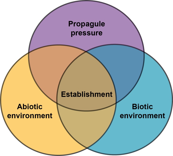
Figure 1: The three main elements governing the likelihood of establishment of exotic species in the introduced region (Derived from Camac et al. 2024)

Biosecurity Commons allows users to create risk maps that account for all, or a subset of the above three constraints, providing critical functionality that can be applied to any threat. It does this by providing access to a wide range of climate, environmental and social (e.g. human population, points of entry) geospatial datasets that can be easily used to construct estimates of climate suitability, biotic suitability or how entry risk may vary across geographic space for different pathways.

For more details about the risk mapping workflow please see the Risk Mapping workflow overview support article. A demonstration video is also available for this workflow.

Linkages to other workflows

Outputs of Risk Mapping can be used directly as inputs in many other workflows, such as:

• Informing Dispersal Modelling by:
  1. Stochastic seeding of incursions based on establishment likelihoods
  2. Constraining geographic spread based on threat suitability
  3. Constraining carrying capacity based on threat suitability (in population spread models)
  4. Informing location attractiveness via threat suitability
• Informing Surveillance Design for early detection by identifying areas of high establishment likelihood
• Informing Proof of Area Freedom by combining risk mapping and surveillance design to determine confidence or likelihood of threat absence.

Creating a Risk Map

Step 1. Create a new project

Select the Risk Mapping workflow and you’ll be taken to the “Create a new Project” section (see screenshot below).

When creating a new risk mapping project, users can create an empty project or one of a range of pre-populated case studies that have been constructed as examples of the workflow or based on previous case studies (e.g. “Mouse-ear hawkweed (Pilosella officinarum)”).

The empty template is ideal for those wishing to create a brand-new risk map as it contains:

• The basic structure of the Risk Mapping workflow
• No preloaded datasets (except for the default region, albeit this can be easily changed) 

In contrast, the example case studies allow users to explore fully worked demonstrations of how establishment-potential maps can be generated. When based on real-world case studies, they also illustrate how others have approached the development of these maps in practice. Users can then adapt and modify these pre-populated templates to suit their own species, regions, or analytical needs.

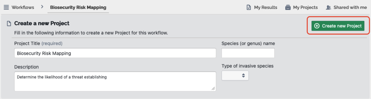
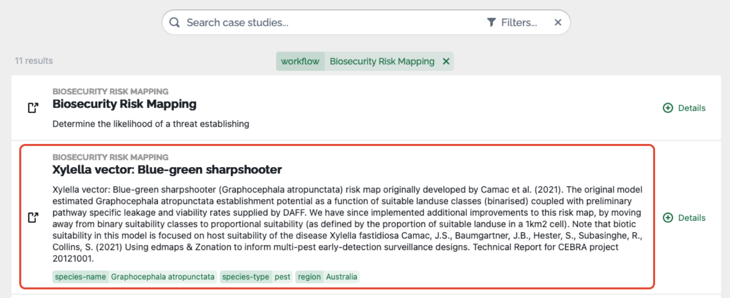
Select a case study and then give your project a title. Users can optionally provide additional descriptive details under the Description, Species name and Species type fields. These metadata are presently unused but will provide future flexibility in filtering and summarising projects.

Once details have been provided, click the green “Create new Project” button to continue.

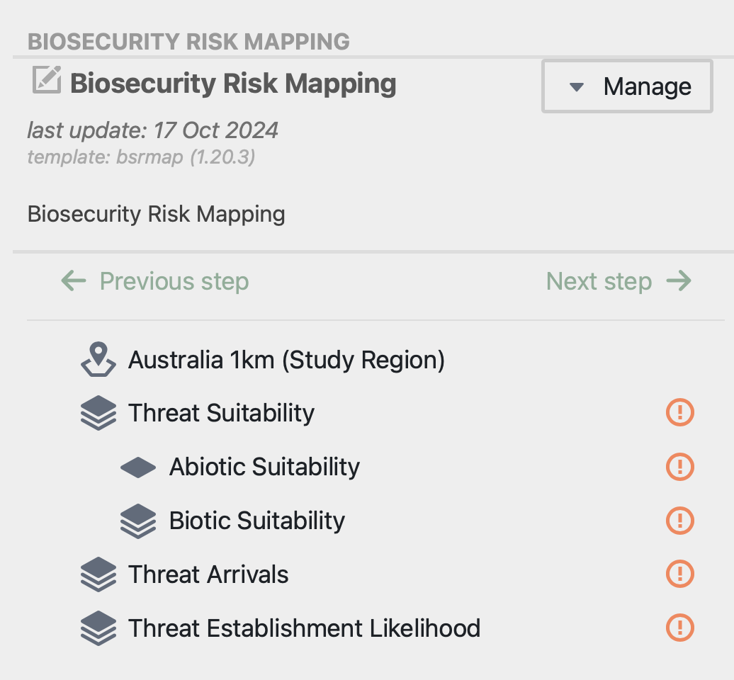
When you start a Risk Mapping workflow from an empty template you will be presented with the core elements of the workflow on the left side of the screen – Study Region, Threat Suitability (which comprises Abiotic & Biotic Suitability), Threat Arrivals and Threat Establishment Likelihood. Orange exclamation points indicate steps that require attention and, as you progress through the project, these change to green ticks when complete.

Step 2. Choose your study region

By default, Biosecurity Commons will load a template raster encompassing the extent of Australia, at 1km resolution, to define the study region. However, this can easily be changed using a variety of options. 

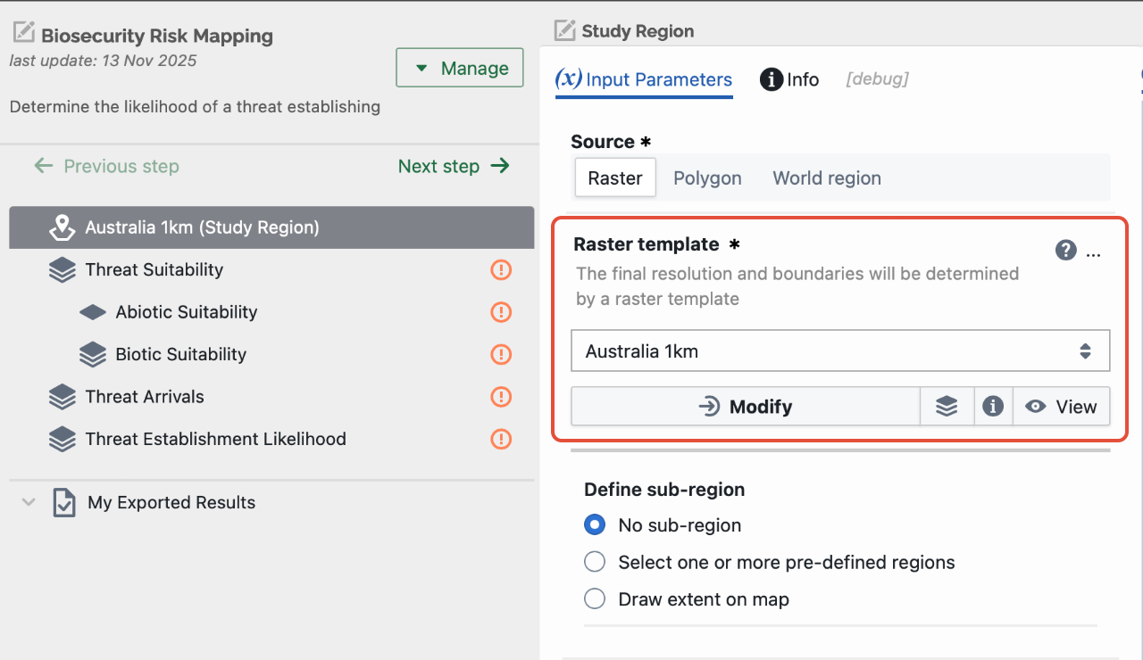
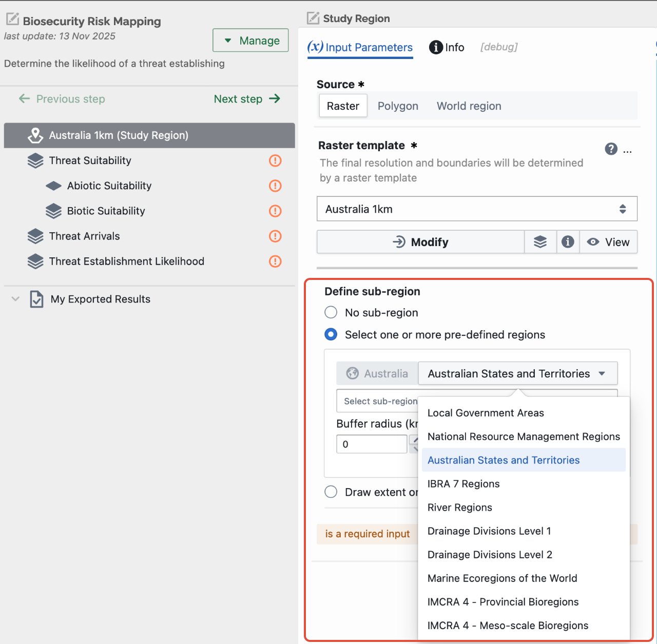
1. Select from a range of pre-determined regions within Australia

By simply selecting “Select one or more pre-defined regions” users can select from a range of predefined regions include: 

• Local Government Areas
• National Resource Management Regions (NRMs) 
• Australian state and territories 
• IBRA regions
• River regions 
• Drainage Divisions (Level 1 or 2)
• Marine Ecoregions of the world
• IMCRA provincial or meso-scale bioregions

For more details about these and other datasets please consult the Atlas of Living Australia.

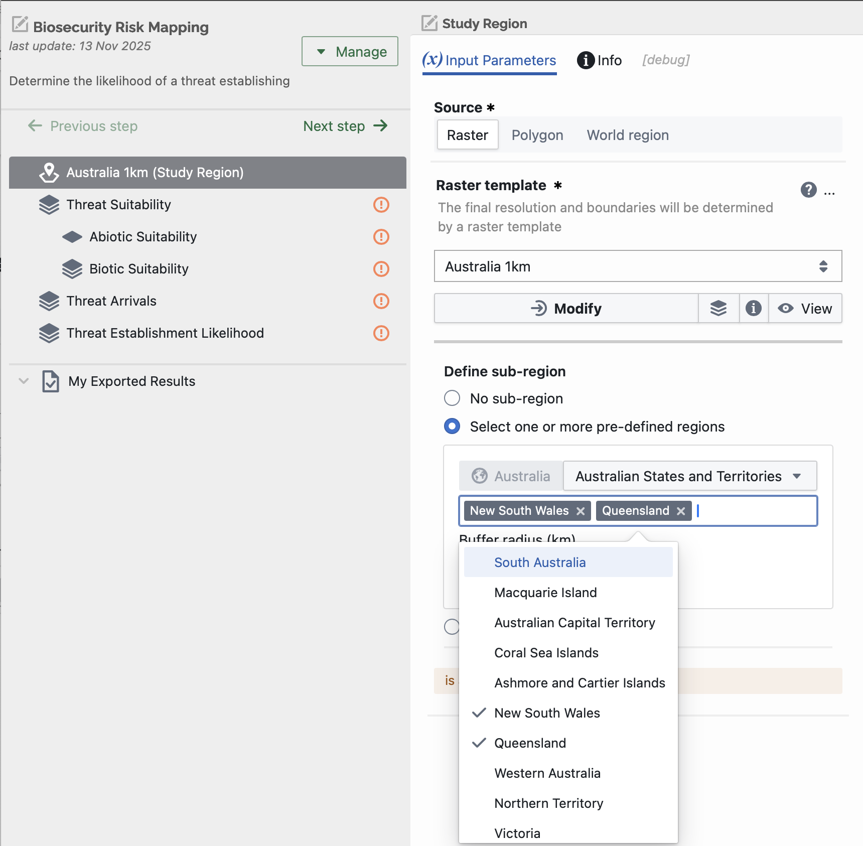
Once selected, users can then specify one or more subclasses to define their study region. For example, if a user selected “Australian States and Territories” and they wished to constrain their study region to Queensland and New South Wales, they can simply select both states from the dropdown menu.

Once selected, users can also add a buffer (units in km) to their pre-defined regions. Adding a buffer can sometimes be useful to ensure complex boundaries (e.g. coastlines) are appropriately captured within the study region.

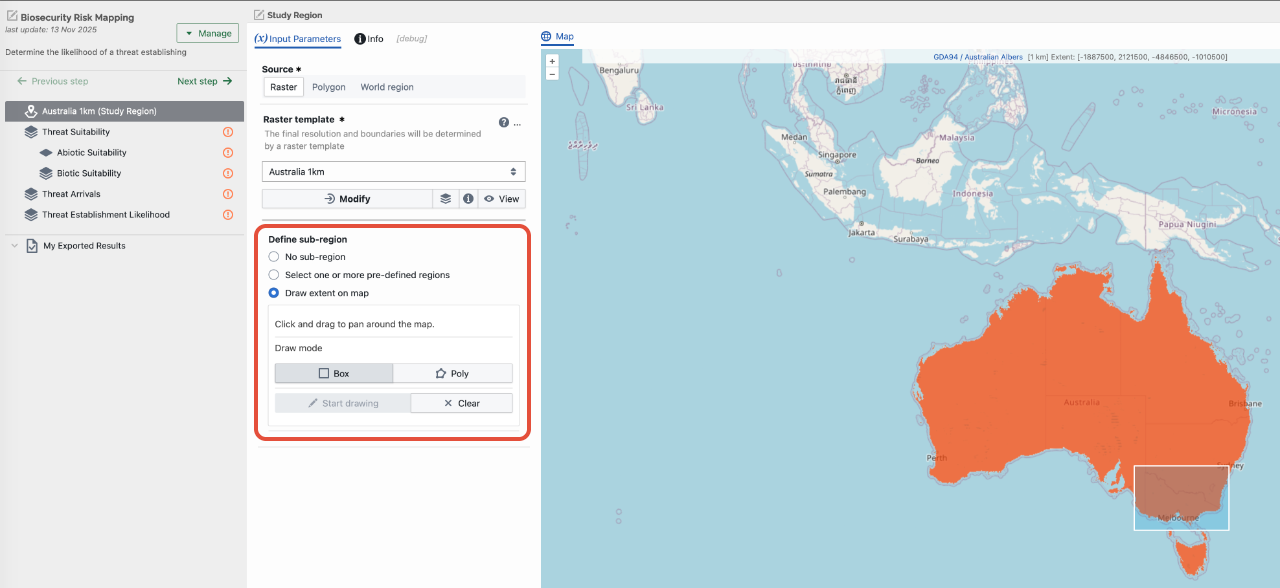
Where a predefined region is not available users can manually draw their extent on the provided map. To do this, select “Draw extent on map”. Users can then either draw a box around the region of interest or draw their own complex polygon over the region of interest. Simply specify the draw mode (Box or Poly) required, then press “Start Drawing”. Then draw your extent on the map the map provided. If you wish to undo a drawing, simply press “Clear”.

1a. Define Region Template

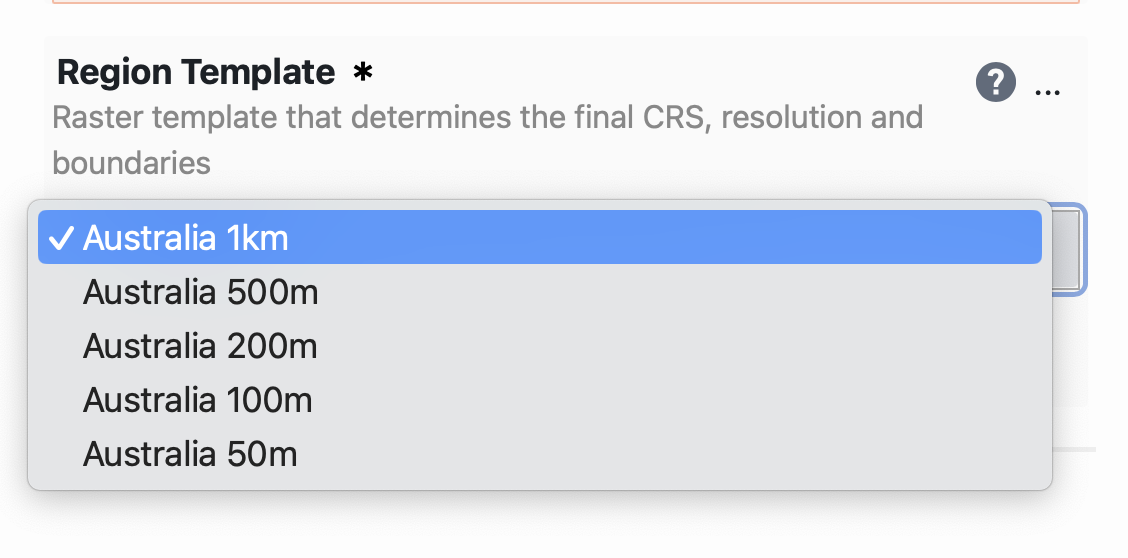
Irrespective of whether a pre-defined or drawn extent is used, users must specify the study region coordinate system and resolution that the workflow will use to construct the risk map. This is specified under the subheading “Region Template”. 

By default, Biosecurity Commons uses a 1km Australian Albers (equal area) projection layer. Extents are rasterized using the coordinate system and resolution defined in “Region Template”.

Users can select a finer Australian Albers template from the dropdown menu.

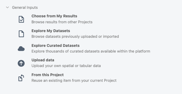
However, if users wish to use a different coordinate system, they are required to click the "Modify" button and then select "Remove input" and then select the “Add New Input” button. From there users can select a raster with the desired coordinate system and resolution either from previously uploaded datasets or results, or from existing curated datasets, or else upload a new raster for this purpose using the import/upload option.

2. Choose your own study region

Users may also opt to specify their own study region by providing the workflow with an existing raster object. In the “Select an alternative input” menu, accessible through the "Modify" button, users have several ways to choose their own study region raster (see screenshot below).

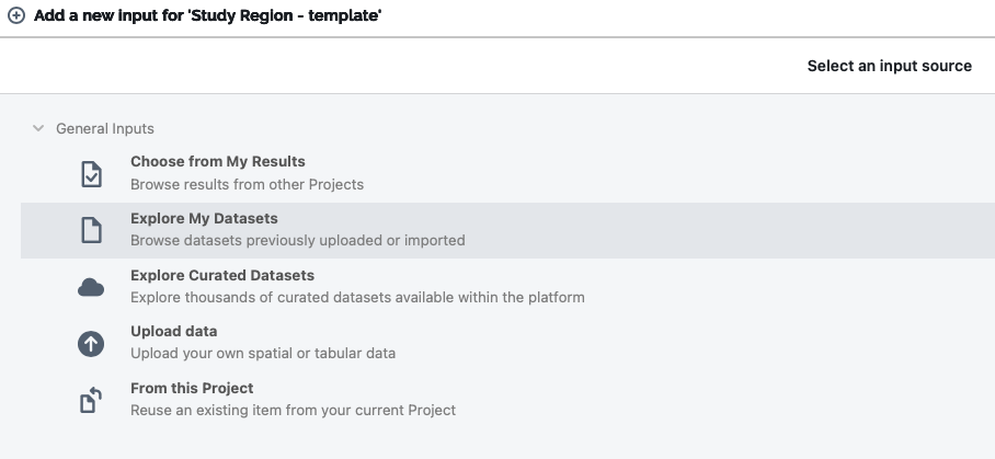
• Choose from My Results: Choose a study region from your results if you have completed previous projects.
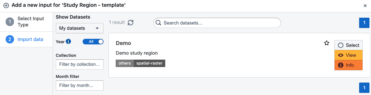
• Explore My Datasets: To search for datasets you have previously uploaded. This will load a window allowing you to search through datasets you have previously uploaded. Once the relevant dataset is selected, simply click “Select” to the right of the dataset, and then click the blue “Add” button in the bottom right of the screen.
• Explore Curated Datasets: Search the curated datasets available on Biosecurity Commons. Given the vast number of datasets provided by the platform, we strongly recommend using the filtering functionality to navigate for appropriate datasets. Once the relevant dataset is selected, simply click “Select” to the right of the dataset, and then click the blue “Add” button in the bottom right of the screen.
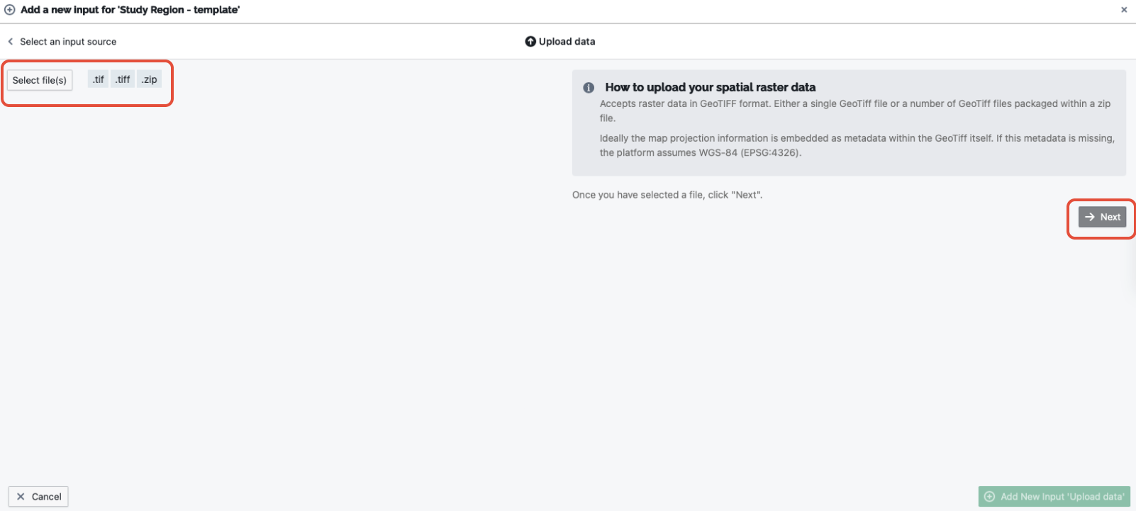
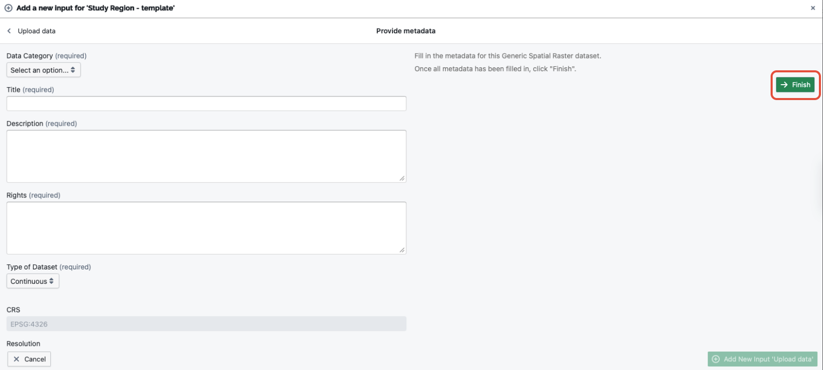
• Upload data: Use this option to upload your own study region in GeoTIFF format. Select this option and then choose the file you want to upload. Click the “Next” button and then you will be required to add a title, description, and information regarding the rights associated with the dataset (see second screenshot below). Finally, click “Finish” and your dataset will be imported (see third screenshot below). Select the uploaded dataset and then click the blue “Add new Input” button.
  
  

Step 3. Threat Suitability

The Threat Suitability step is by default made up of two components:

• Abiotic suitability: A spatial layer that defines the suitability of the abiotic environment (i.e. non-living factors such as climate) that may be conducive for threat survival and establishment
• Biotic suitability: A spatial layer that defines the suitability of the biotic environment (i.e. living environment, such as habitat or host availability) that may be conducive for threat survival and establishment.

While both factors are often critical barriers to threat establishment, there may be cases where a threat may not be exposed to ambient climatic conditions (e.g. pests of stored produce) making the abiotic environment an unnecessary component. Alternatively, some Species Distribution Models may explicitly account for both biotic and abiotic factors, and thus, remove the need to separate both forms of suitability.

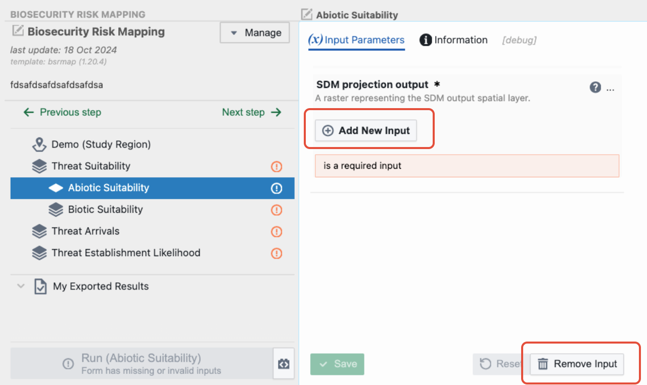
If only one of these two factors is relevant, the platform allows users to easily remove a factor. To do this, simply select “Abiotic Suitability” or “Biotic Suitability” and then click “Remove Input” at the bottom of the screen. This will remove the requirement for this component to be completed within the workflow.

NOTE: The risk mapping workflow combines abiotic suitability, biotic suitability, and arrival pathways by multiplying the layers together. It is therefore important to carefully consider how each layer is constructed and the values it contains. Using the approach specified in Camac et al. 2021, each layer should ideally represent the relative probability of either suitability or arrival. Thus, each component should be on the proportional scale if assuming equal weighting of components. To maximise flexibility in use (and allow for differential weighting to each component), Biosecurity Commons does not enforce these layers to be bounded between (0 and 1). 

In the following sections, we briefly outline how each suitability component can be defined and included in a risk map workflow.

1. Abiotic Suitability

In most cases, the abiotic suitability layer refers to the climatic suitability for a threat. Commonly this is derived from some form of species distribution model. 

Within the risk mapping workflow, users can define this component in four primary ways: 

• Create a new abiotic layer using SDM functionality within the risk mapping workflow
• Import an existing SDM created in a SDM project
• Upload a SDM output built off-platform, or import from “Curated Datasets” or “My Datasets”
• Create a custom suitability layer by combining spatial layers using Toolbox Functionality

1a. Create a new Species Distribution Model (SDM) within the Risk Mapping workflow

The first option is to fit a SDM directly within the risk map project. To do this, select “Create a new Species Distribution Model (SDM)” and then click the blue “Add New Input” button.

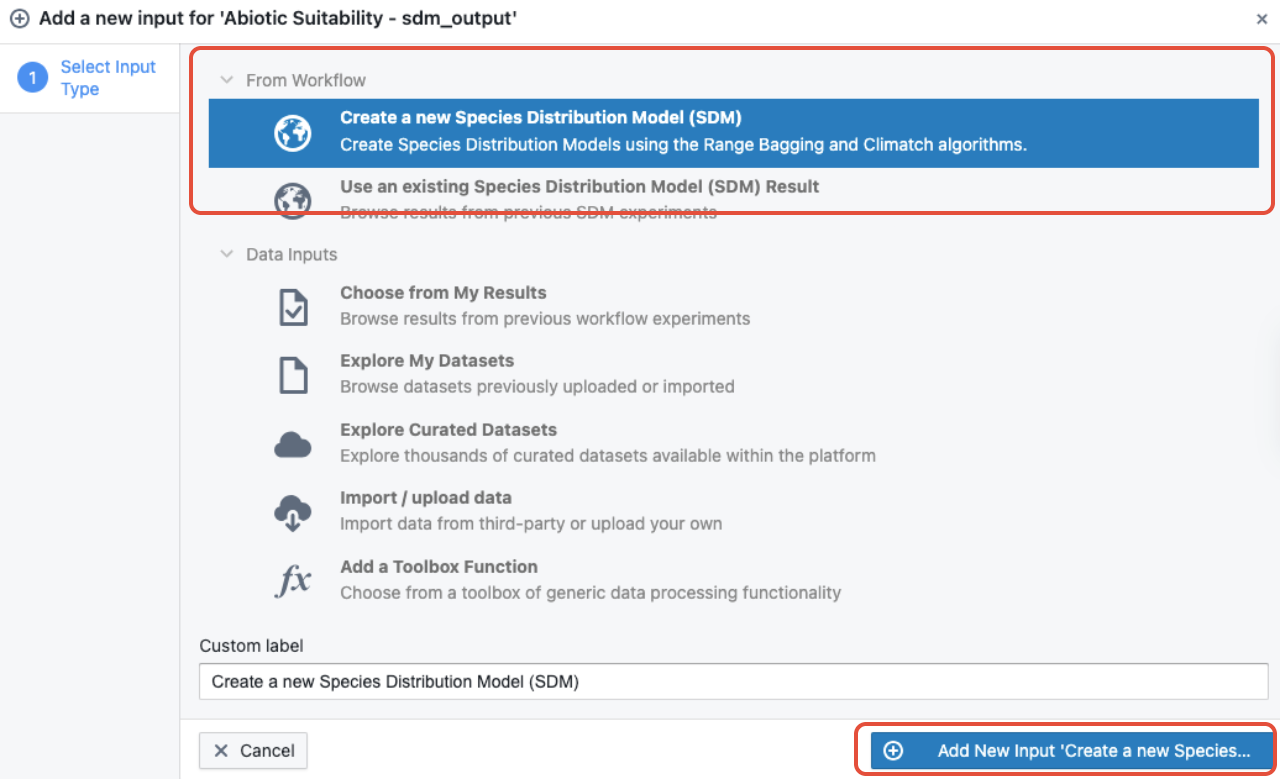
This feature allows users to create a SDM within the Risk Mapping workflow. When selected, several sub-steps will appear in the tree (see screenshot below).

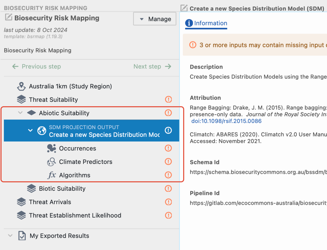
To produce a successful SDM, please follow the instructions in our SDM start guide.

1b. Use an existing Species Distribution Model (SDM) result

The second option is to import an existing SDM project output created on Biosecurity Commons. To do this, select “Use an existing Species Distribution Model (SDM) Result” and then click the blue “Next” button.

This allows users to choose a SDM from their results. Find the relevant project, click on it and then select the output file named “Projection to current climate – unconstrained". Once this is done, click the blue “Add New Input” button. This will import the SDM into the Risk Mapping workflow.

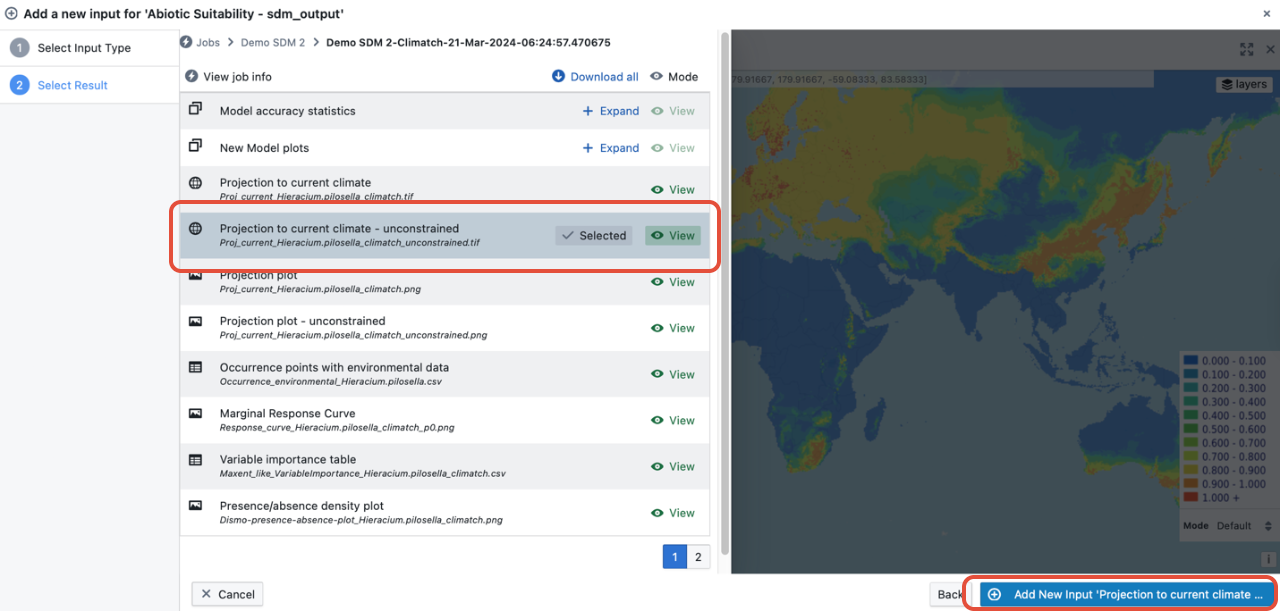
1c. Upload a SDM output built off-platform or import from “Curated Datasets” or “My Datasets”

If a user has created a SDM file offline or off-platform, it can be uploaded and used within the risk mapping workflow by doing the following:

“Select Add New Input” > “Import / upload data” > “Upload my own data”, then specify the data type (often Generic Spatial Raster) and upload a GeoTIFF of your abiotic suitability layer.

Alternatively, as in most cases, users can explore their own previously uploaded datasets or available curated datasets for specifying abiotic suitability.

1d: Create a custom suitability layer by combining spatial layers using Toolbox functionality (ADVANCED USERS)

Biosecurity Commons also provides advanced users the ability to combine and modify existing raster objects in many ways to construct new spatial objects that can be used in a variety of contexts, including informing abiotic and biotic suitability. To use this functionality, select “Add a Toolbox Function”.

Users will then be able to select from a range of raster manipulation options (see below).

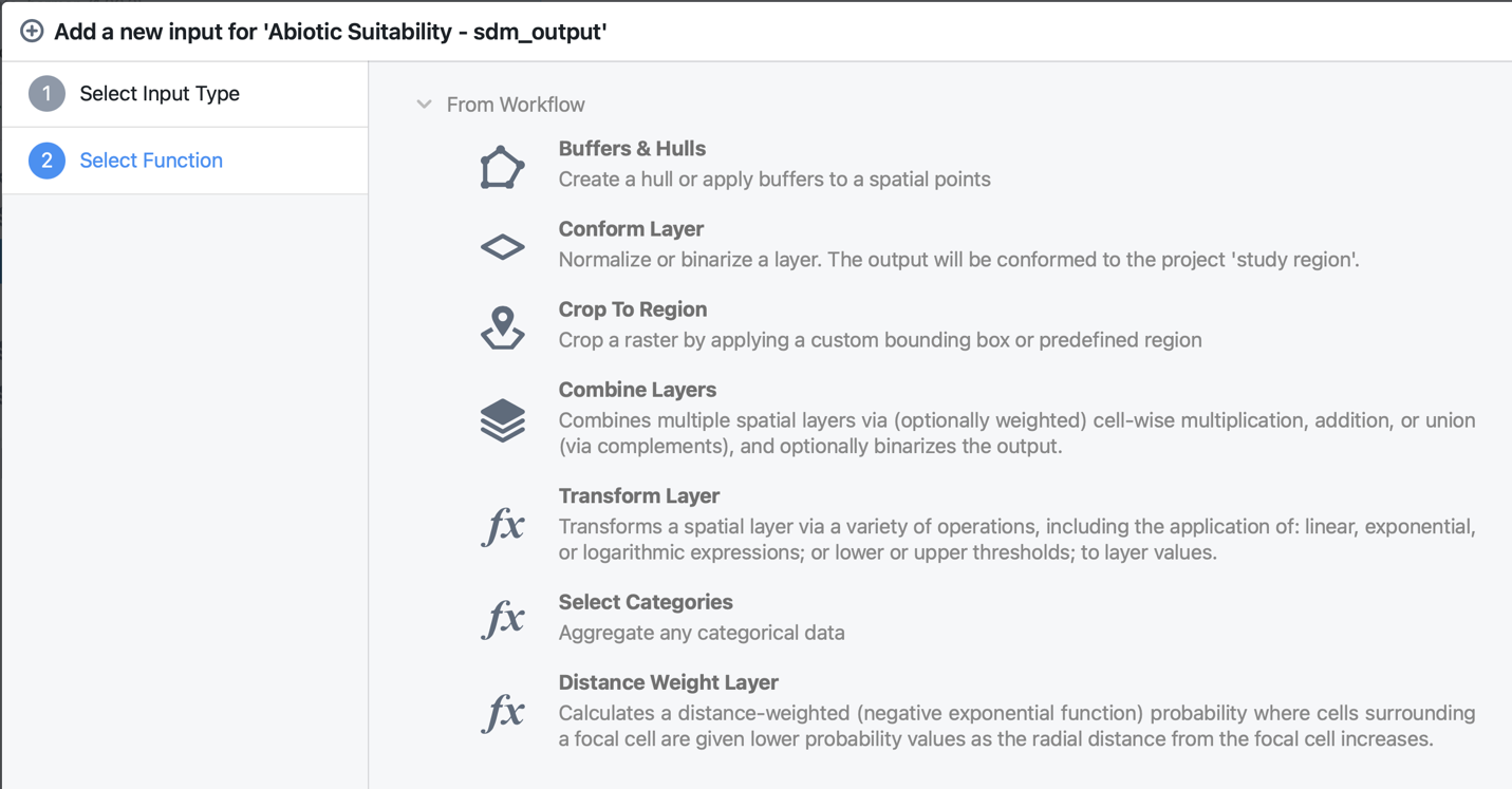
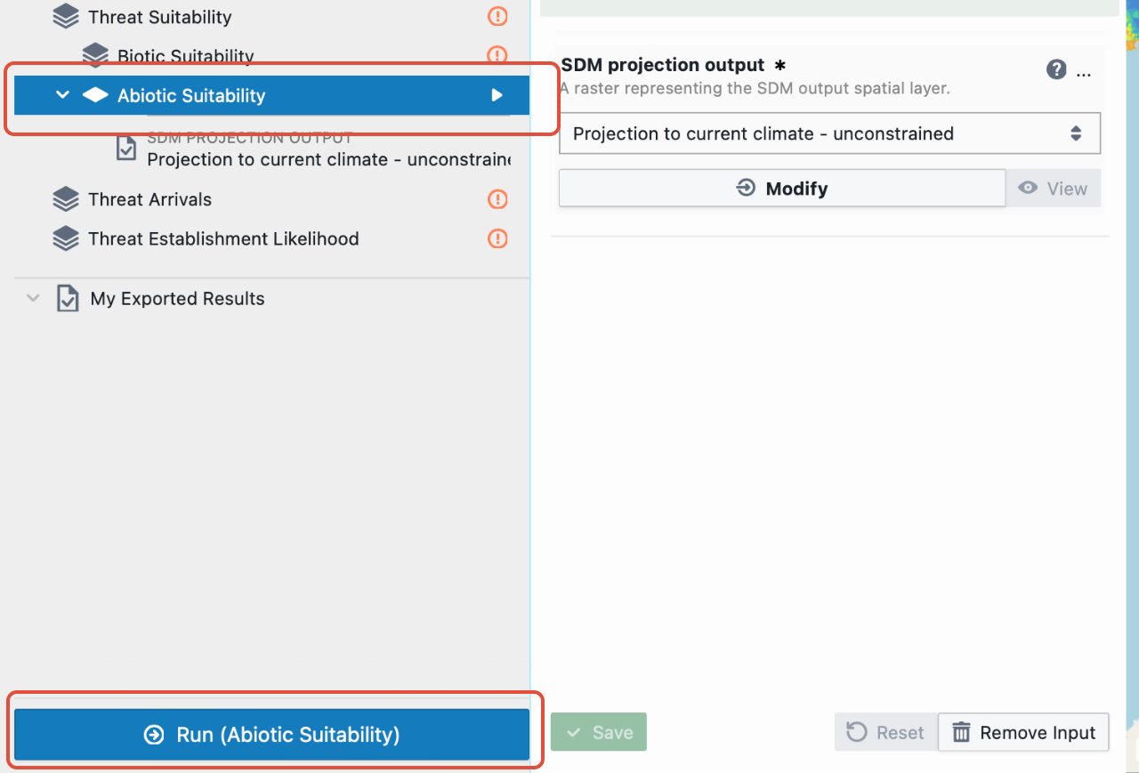
Once a user has specified their abiotic layer and pressed the green save button, they can then click the “Abiotic Suitability” tab on the left-hand panel and click the “Run” button in the lower left-hand corner to complete this step in the tree (see screenshot below).

2. Biotic Suitability

Biotic suitability often refers to the suitability of the living environment at a location. This can be defined in many ways, including:

• Fitting a separate SDM for a host species, or habitat type
• Inferring suitability based on vegetation or land use or other landscape attributes

Broadly the biotic suitability component follows a similar path as the abiotic suitability section stepped through above. However, there are a few unique differences.

First when users select biotic suitability and then select “Add New Inputs”, they have easy access to high resolution land use and vegetation classification rasters that are commonly used in biotic suitability approximations (see below).

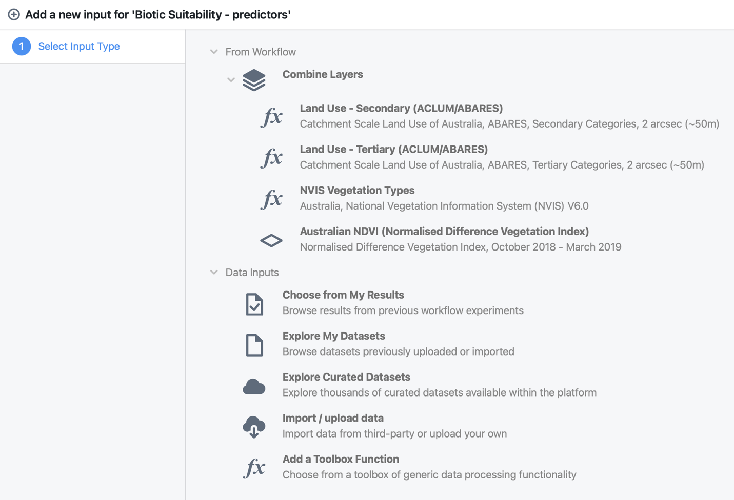
Users can select one or more of these, explore datasets in either “My Results” or “Curated Datasets” or import a new dataset in the same way as is described above and is commonly done elsewhere on the platform.

The key distinction with biotic suitability is that it allows users to easily convert one or more multi-class rasters into a raster that can be used to inform biotic suitability.

For example, if a user selects “Land Use – Secondary (ACLUM/ABARES)” as an input, they will then be prompted to select suitable classes (see below).

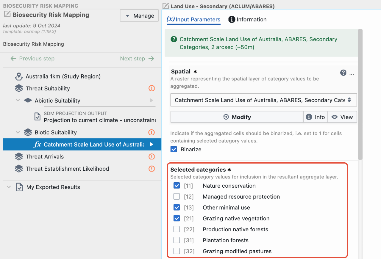
In addition to checking the categories that are deemed suitable for the threat, users can also define whether they want to create a binary (i.e. suitable versus unsuitable) raster or calculate the proportion of area containing suitable land classes at the defined Study Region resolution. 

Checking the Binarize tick-box will convert all selected classes to 1, and all non-selected classes to 0 in the grid cells of the map. If Binarize is not selected it will calculate the proportional area containing suitable land use types (in this case the fraction of each 1km² cell that is comprised of suitable 50m² cells, since the land use raster has 50m² resolution and the study region has 1km² resolution).

NOTE: If users are constructing a biotic suitability layer as a function of multiple input rasters, they should carefully inspect the “Use function” argument, which defines how multiple objects will be combined.

Currently three options are available:

• Prod – Multiply the layers together (Most commonly used option)
• Sum – Sum the layers together
• Union – Calculate the union via 1 – prod(1 – x). This is mostly used for probability layers where one is interested in calculating the likelihood of one or more layers being suitable.

If users wish for the combined output to be binary, they can select “Binarize”. This will binarize across layers and assign 1 to any non-zero/non-NA cell value.

Once the biotic suitability layer has been defined, click Save and then click Run.

When the function has run successfully, the orange exclamation mark next to your layer in the tree will turn into a green tick. 

You can also click the “Export to ‘My Results’” button, which will appear next to the Run button after the layer has run successfully. 

This allows users to add this layer to the “My results” section of their dashboard. From this section users may download this layer, make it available for use in other workflows, or share it with other registered users of Biosecurity Commons. Users can also view or download the R script used to generate the layer, the log file, the metadata, or the input parameters json file.

Finally, click on the Biotic Suitability step in the tree and select the blue “Run” button to complete this step.

3. Threat Suitability

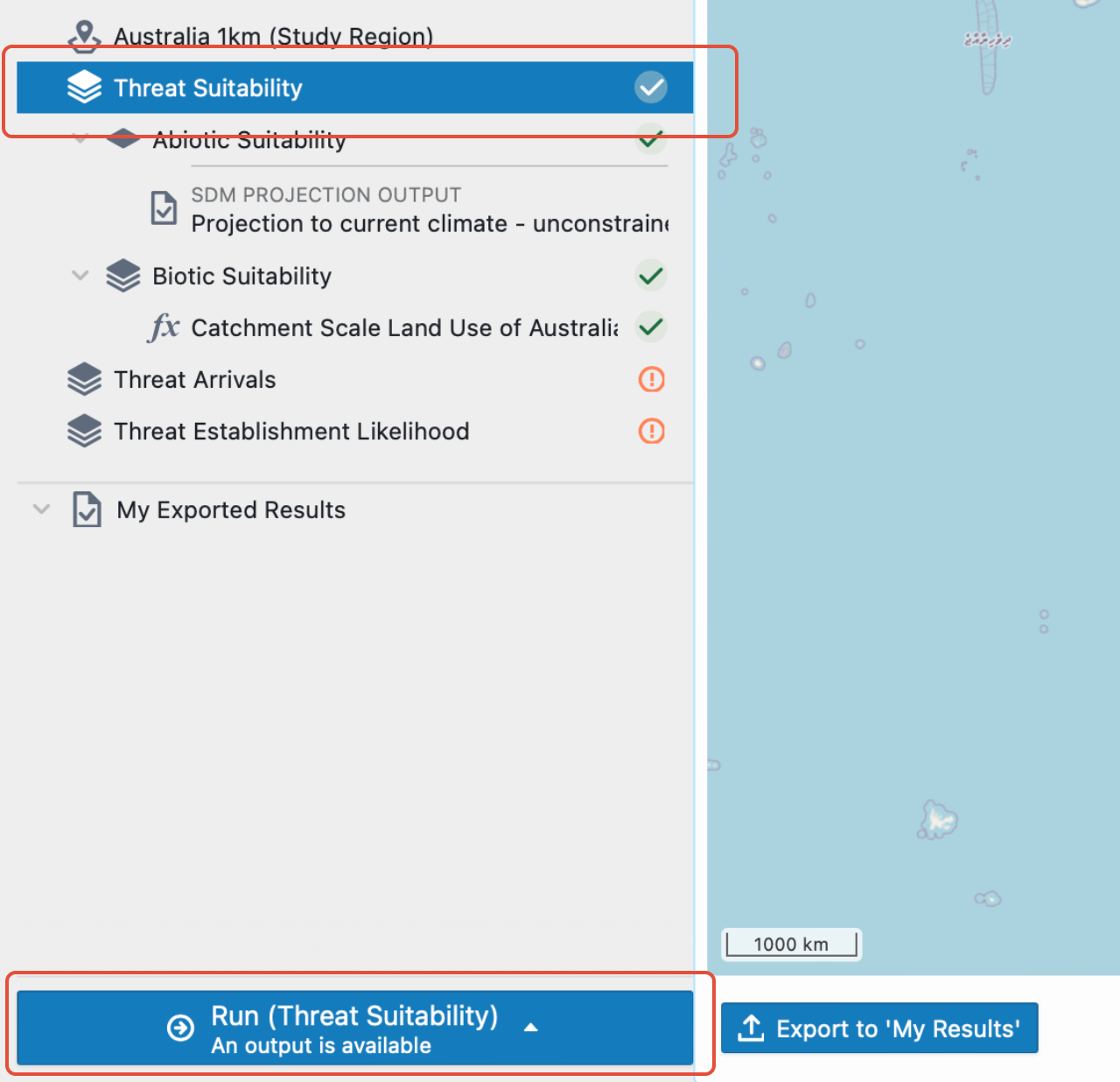
Once the mandatory abiotic and biotic suitability functions have run successfully (green tick), or have been removed (if not required), select “Threat Suitability” in the tree and run the function to complete this stage (see screenshot below).

Step 4. Threat Arrivals

The fourth step involves approximating the likelihood of an arrival event in each location (i.e. the propagule pressure).

While this component is included by default, users may remove this input the same way as they can remove the abiotic or biotic component, by simply selecting the branch (i.e. Threat Arrivals) and then selecting “Remove input”.

However, if users wish to account for likelihood of arrival, they can add relative weighting layers for one or more pathways of entry.

Simply click “Add New Input” to add one or more threat arrival layers, representing the different modes of entry into Australia. Users will then see the menu in the screenshot below which provides the option of adding predefined curated functions for pest arrivals. These predefined options are derived directly from Camac et al. 2021 (see below).

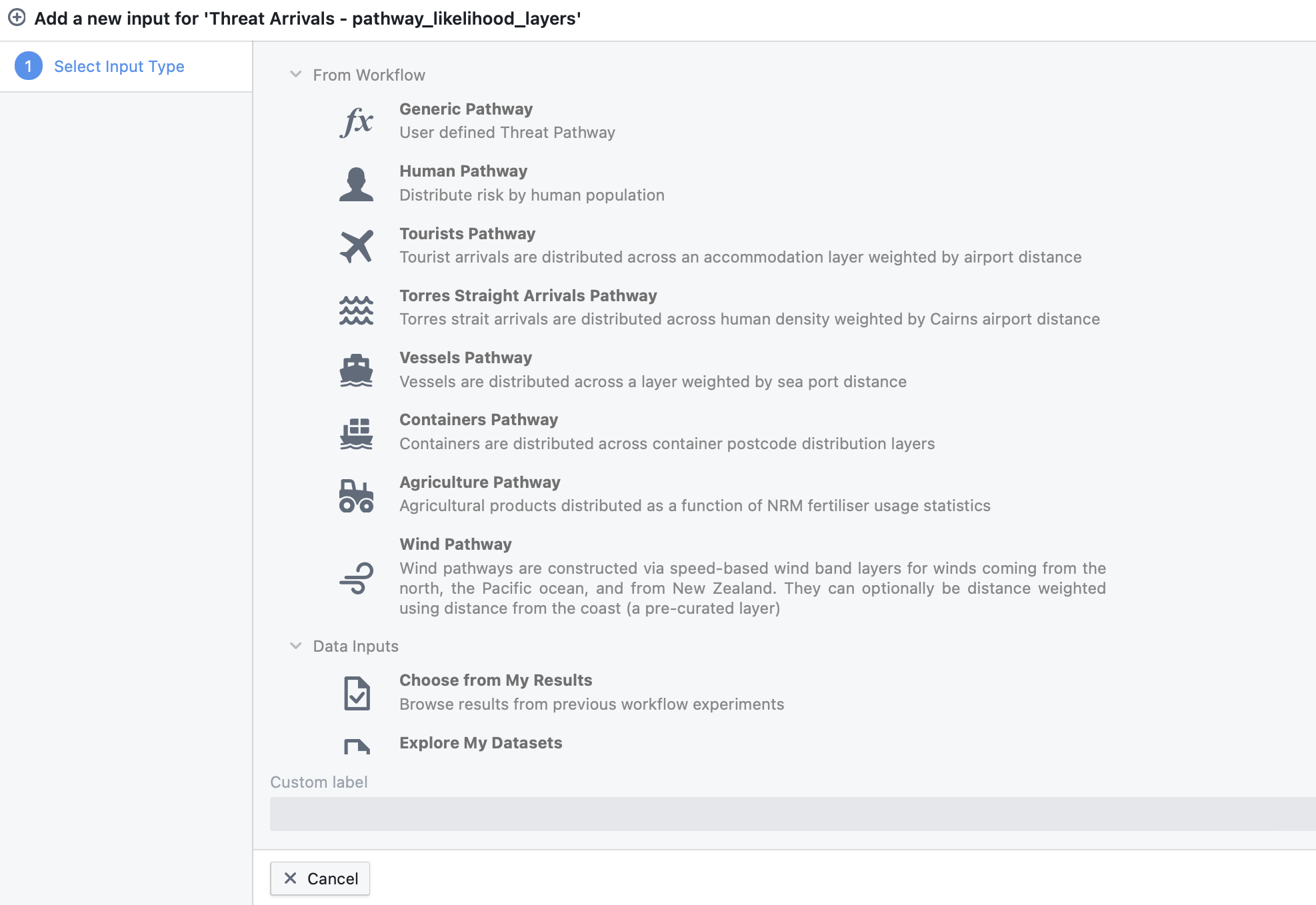
Users can also create their own custom raster for distributing pathway risk by selecting Generic Pathway, which will prompt the user to specify one or more weighting rasters.

In the example below (see screenshot), the Tourists Pathway layer is selected, and a new step appears in the tree. Users can modify the following:

• Pest Pathway layers: A proportional weighting raster for distributing arrivals. In the example below the proportion of human population density is used
• Leakage rate: The lower and upper confidence limits of the expected number of contaminated events per time period (e.g. year) that pass pre-border and border inspection procedures
• Viability rate: The lower and upper confidence limits of the probability that a contaminated item that passes border inspection procedures is viable for potential establishment (prior to considering abiotic and biotic suitability of the arrival destination)
• Confidence interval: the confidence level associated with the lower and upper confidence limits provided above (default 0.95)
  
  

For more details about these parameters, please consult the risk mapping support material.

To the right of the parameters is a graph showing the expected number of viable leakage events based on leakage and viability inputs derived from 100,000 stochastic samples. The probability above the graph signifies the probability that one or more viable leakage events occur. The graph dynamically updates as inputs change. 

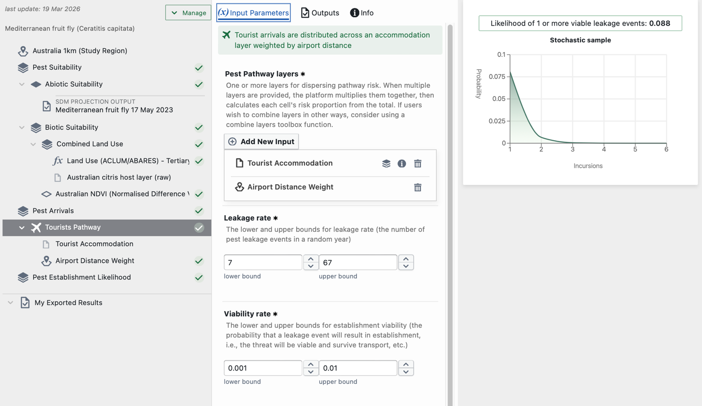
After updating the parameters, click “Save” and then “Run” the function to generate the result. If successful, the Human Pathway layer will show a green tick. 

This step can be repeated for any of the other pathway options available. 

Finally, to complete this section of the tree click on “Threat Arrivals” and then click on the blue “Run” button to turn the exclamation mark to a green tick.

Step 5. Threat Establishment Likelihood

Once the Threat Suitability and Threat Arrivals functions have been successfully run you will be able to run the overall Threat Establishment Likelihood function (see screenshot below). 

Click the blue ‘Run’ button in the bottom left to run your project. The output page will be updated as the job progresses from “Created”, “Submitted”, “Started” and “Success”.

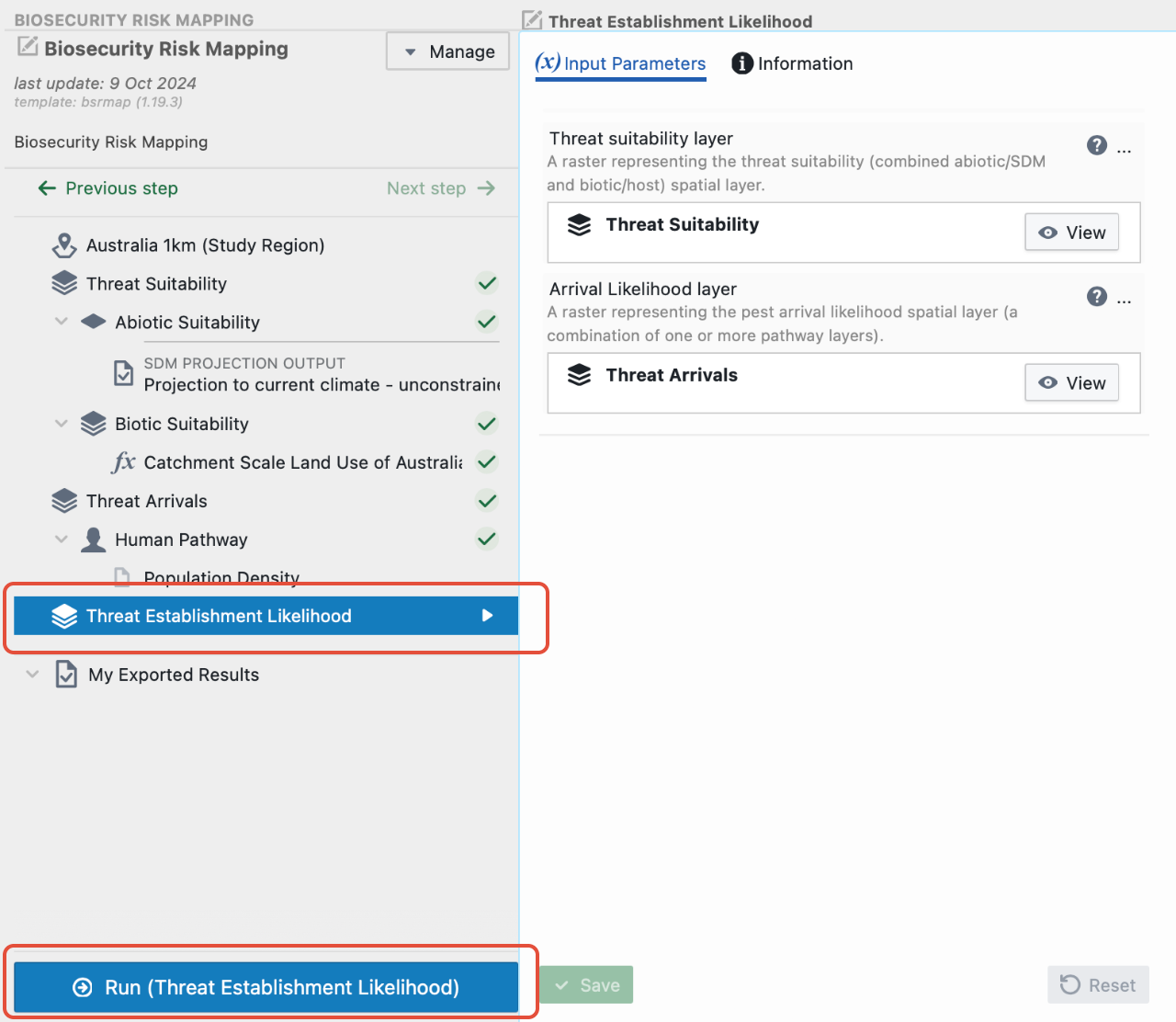
Once it has finished, a green tick will appear next to Threat Establishment Likelihood. 

The model output will automatically be displayed as a viewable risk map in the interactive map pane (screenshot below). Users can zoom in or out of regions of interest. Interactive maps also allow users to change the type of legend displayed.

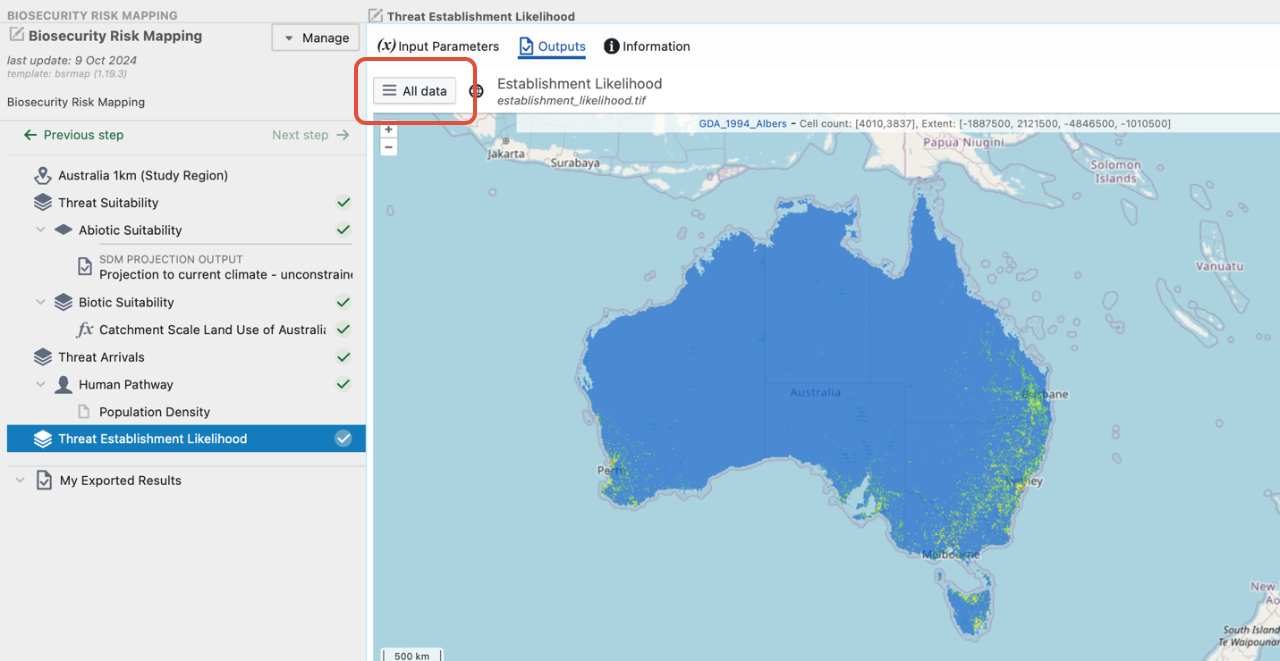
Clicking on the “All data” button allows users to view and download all the outputs. 

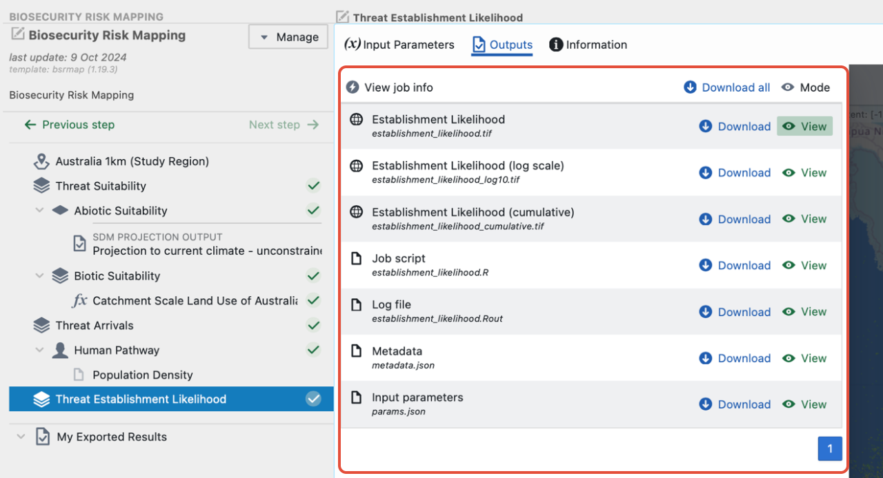
These outputs include:

• Establishment Likelihood: The relative likelihood of establishment conditioned on threat suitability and/or Threat arrivals
• Establishment Likelihood (log scale): The relative likelihood on the log10 scale. Useful for viewing exceedingly small probabilities
• Establishment Likelihood (cumulative): Calculated by ranking raster cells based on their establishment likelihood and then computing the cumulative sum so that each cell’s value represents the likelihood of threat establishment in that cell or any cell with a higher likelihood. Useful for highlighting locations with highest risk of establishment
• Job script: A copy of the R script used to build the risk map
• Log file: A text file containing processes, messages, and other details associated with model runs
• Metadata: A .json file containing the metadata required to run the model on Biosecurity Commons
• Input parameters: Input parameters required to run the Job Script

Step 6. Exporting outputs for use in other workflows

Users may wish to export outputs for use in other projects or other workflows.

To do this, view the output of interest, and select “Export to My Results” in the bottom left corner of the interactive map. 

This output will now be discoverable in the user’s “My results” database, which in turn makes the layer available for use in other workflows.