Population Spread modelling

Overview

Following introduction into a new region, invasive pests, weeds, and diseases rarely remain confined to their initial point of establishment. Instead, populations establish, grow, disperse, colonise new areas, and may continue expanding until constrained by environmental conditions, resource availability, management interventions, or other demographic and ecological processes. Understanding how an invasion develops through space and time is therefore fundamental to biosecurity preparedness, surveillance, response, and long-term management.

Population Spread Modelling simulates these invasion processes by representing how populations establish, grow, disperse, colonise new locations, and respond to management over successive simulation time steps. Unlike static risk maps, which estimate where a species could establish if introduced, spread models explicitly simulate the dynamic progression of an invasion following establishment, allowing users to estimate both where and when a species is likely to spread under alternative biological assumptions and management scenarios.

Unlike many population models developed for specific organisms or applications, the Population Spread Modelling workflow is intentionally flexible. Rather than prescribing a single modelling approach, users progressively construct a spread model by selecting how space, population dynamics, dispersal processes, impacts and management actions should be represented. This allows the workflow to be adapted to a broad range of biosecurity questions, organisms and data availability.

Population spread models support a wide range of biosecurity applications, including:

• Forecasting the spread of newly established pests, weeds and diseases.
• Estimating the future extent and timing of invasion.
• Identifying areas likely to be invaded first.
• Prioritising surveillance, containment and eradication activities.
• Evaluating alternative management strategies.
• Estimating how economic, environmental and social impacts may accumulate through time.
• Supporting evidence-based preparedness and resource allocation.

Unlike many analytical workflows within Biosecurity Commons, Population Spread Modelling is inherently dynamic and stochastic. Each simulation represents one possible realisation of the invasion process based on the specified biological assumptions, parameter values, dispersal processes and random events. Consequently, multiple replicate simulations are typically required to characterise uncertainty and estimate quantities such as expected population abundance, probability of occupancy, and time of arrival.

Rather than providing a single predefined spread model, Biosecurity Commons provides a flexible modelling framework that allows users to combine alternative representations of space, population dynamics, dispersal processes, impacts and management actions to construct models tailored to their specific biosecurity question. Depending on the management question and available data, simulations may represent spread across continuous landscapes using raster models, between discrete locations using network models, or without explicit geography using spatially implicit models. Likewise, populations may be represented using presence-only, unstructured or stage-structured population models.

Population Spread Modelling is closely integrated with other Biosecurity Commons workflows. Outputs from the Establishment Likelihood workflow is used to define spatial variation in establishment probability and, where appropriate, modify population growth according to landscape suitability. Establishment likelihood maps may also be used to seed initial incursions when constructing spread scenarios. Conversely, outputs from Population Spread Modelling can inform Surveillance Design, Resource Allocation, Impact Analysis and Proof of Freedom workflows, allowing users to iteratively evaluate invasion scenarios, surveillance strategies and management interventions within a consistent analytical framework.

The quality and realism of spread model predictions ultimately depend on the biological assumptions, parameter values and input datasets used to construct the model. Consequently, exploring alternative scenarios and conducting sensitivity analyses are often as informative as any individual simulation. Throughout this support article, emphasis is placed not only on how each modelling option functions within Biosecurity Commons, but also on when it should be used, the assumptions it makes, and the implications those assumptions have for interpreting simulation results and supporting evidence-based biosecurity decision-making.

Choosing a Spatial Modelling Framework

The first and arguably most important decision when constructing a population spread model is selecting how space will be represented. This decision determines not only how populations move through the landscape, but also the types of biosecurity questions the model can answer, the input data required, the computational complexity of the simulation, and the interpretation of model outputs.

Biosecurity Commons supports three complementary approaches for representing space:

• Raster (Grid) models, which represent the landscape as a continuous grid of cells.
• Network models, which represent the landscape as a collection of discrete locations connected by movement pathways.
• Spatially implicit models, which simulate changes in population size or occupied area without representing explicit geography.

Raster, network and spatially implicit models are not different spread models. They are different ways of representing space. Once the spatial framework has been selected, the remaining model components—including population dynamics, dispersal, impacts and management actions—are configured in much the same way.

None of these approaches is universally better than the others. Instead, each is designed to address different classes of biosecurity problems. Selecting the most appropriate framework depends on the biology of the organism, the dominant mechanisms of spread, the available data, and the management question being addressed.

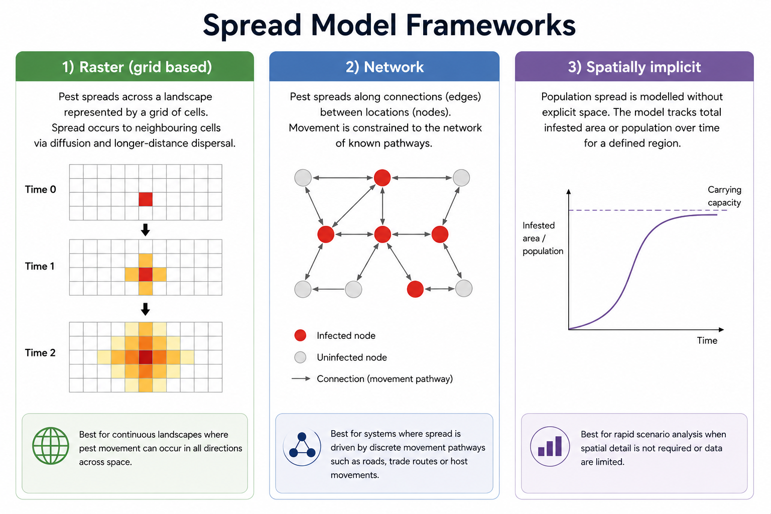
Which spatial modelling framework should I choose?

Raster (Grid) Models

Raster models represent the landscape as a regular grid of cells, with each cell describing a small area of the study region. Populations establish, grow and disperse between cells over successive simulation time steps. Each cell may also contain additional information such as establishment probability, carrying capacity, management actions, or environmental suitability.

Raster models are the preferred approach whenever the movement of an invasive species is influenced by continuous environmental variation or when understanding where spread is likely to occur is an important management objective (e.g. Williams et al. 2008; Bradhurst et al. 2021).

Because most environmental datasets (for example climate, vegetation, land use and host distributions) are available as raster layers, raster models naturally integrate with other Biosecurity Commons workflows, particularly the Establishment Likelihood workflow.

Recommended applications

• Environmental weeds.
• Forest pests.
• Plant pathogens.
• Wildlife diseases.
• Invasive insects.
• National or regional spread forecasting.
• Surveillance planning.
• Delimitation and response planning.

Advantages

• Explicitly represents continuous landscapes. Raster models simulate spread across continuous space, allowing populations to establish, grow and disperse throughout the landscape rather than only between predefined locations. This makes them particularly well suited to environmental pests, weeds and wildlife diseases where spread is not confined to known movement pathways.
• Integrates directly with spatial environmental datasets. Many biosecurity datasets—including climate, host distribution, land use, topography, vegetation and habitat suitability—are naturally represented as raster layers. Raster models can therefore readily incorporate environmental heterogeneity and interact seamlessly with outputs from other Biosecurity Commons workflows.
• Produces intuitive spatial outputs. Raster models generate maps showing the predicted distribution, abundance, probability of occupancy or arrival time of an invasion through time. These outputs are easy to visualise and interpret, making them valuable for surveillance planning, preparedness and operational decision-making.
• Represents heterogeneous landscapes. Biological processes such as establishment, population growth, dispersal and management can vary continuously across space through the use of spatially explicit raster layers. This enables simulations to account for differences in habitat suitability, carrying capacity, movement resistance, management effort or other landscape characteristics.
• Compatible with the Establishment Likelihood workflow. Outputs from the Establishment Likelihood workflow can be used directly within raster spread models to define spatial variation in establishment probability and, where appropriate, influence population growth. This provides a consistent analytical framework linking environmental suitability with invasion dynamics.

Limitations

• Computational requirements increase rapidly with study area size and raster resolution. Every additional raster cell potentially increases the number of locations that may establish, grow or receive dispersers. Consequently, simulation time and memory requirements increase rapidly as study regions become larger or raster resolution becomes finer.
• Large simulations may require computational optimisation. National-scale analyses or simulations performed at fine spatial resolutions can become computationally demanding. In these situations, techniques such as two-tier dispersal can substantially improve performance while preserving the spatial resolution required to represent biologically important local spread.
• Requires careful selection of spatial resolution. The raster resolution should be chosen to represent the ecological processes being modelled and the resolution of the available input data. Selecting an unnecessarily fine resolution increases computational cost without necessarily improving biological realism, while selecting a resolution that is too coarse may fail to capture important landscape features or local dispersal processes.
• May not represent movement through discrete pathways. Raster models generally assume that spread occurs across continuous space according to the specified dispersal process. Where spread is primarily driven by known movement pathways, such as livestock movements, trade networks or transport routes, network models may provide a more realistic representation.
• Dependent on the quality of spatial input layers. Predictions are only as reliable as the underlying raster datasets used to parameterise the model. Errors or mismatches in environmental suitability, carrying capacity, permeability or other spatial inputs can propagate throughout the simulation and influence predicted spread patterns.

CAUTION: MATCH INPUT AND MODEL GRID RESOLUTION

For grid-based models, it is strongly recommended that all spatial model inputs are prepared at the same grid resolution as the Study Region and the resolution at which population and spread dynamics will be simulated.

Biosecurity Commons will automatically resample input rasters that do not match the Study Region grid, using bilinear interpolation for continuous variables and nearest-neighbour resampling for categorical variables. While this allows datasets with different resolutions to be used, resampling can alter the meaning or magnitude of some variables and may produce unintended model behaviour.

This is particularly important for variables representing absolute quantities per grid cell, such as carrying capacity. For example, if carrying capacity is specified for 5 km × 5 km cells but the model operates on 10 km × 10 km cells, simply resampling the carrying-capacity raster does not sum the carrying capacities of the smaller cells. Instead, interpolation estimates a value for each larger cell, potentially resulting in a substantial underestimate of the carrying capacity represented by that area.

Where possible, users should therefore aggregate, rescale or otherwise prepare input layers at the intended model resolution before uploading them to Biosecurity Commons, using an aggregation method appropriate to the meaning and units of each variable.

Network Models

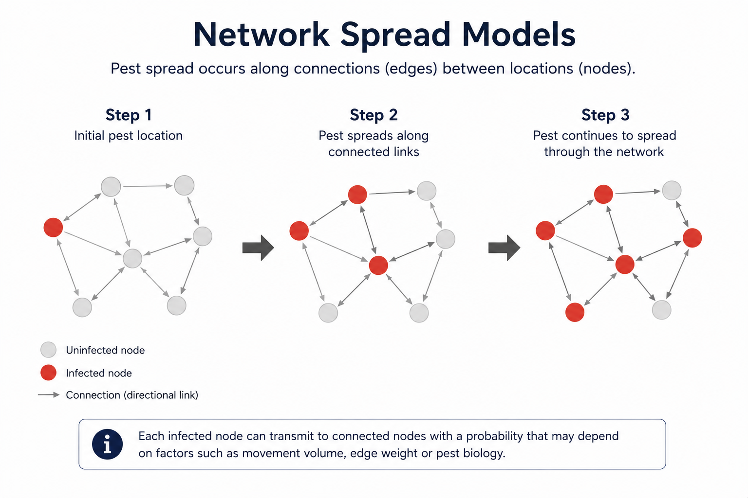
Network models represent the landscape as a collection of discrete locations (nodes) connected by predefined pathways. Rather than simulating spread continuously across the landscape, populations establish, grow and disperse only between these connected locations. This makes network models particularly well suited to biosecurity systems where spread is driven primarily by identifiable movement pathways rather than local environmental diffusion.

Typical applications include livestock diseases spreading between farms (Bradhurst et al. 2015), movement of nursery stock between production facilities, shipping or freight networks, irrigation systems, and movement between isolated habitat patches.

Recommended applications

• Livestock diseases.
• Farm-to-farm spread.
• Nursery and horticultural industries.
• Shipping and freight networks.
• Irrigation and river systems.
• Supply chain and transport networks.
• Movement between isolated habitat patches.

Advantages

• Explicitly represents movement pathways. Network models naturally represent systems where spread occurs between identifiable locations connected by known movement pathways, rather than continuously across the landscape.
• Computationally efficient. Because simulations are performed only between connected locations rather than across every raster cell, network models are often considerably faster than raster models when modelling large numbers of discrete locations.
• Naturally represents discrete management units. Nodes typically correspond to operational units such as farms, orchards, ports or production facilities, making the outputs directly relevant to surveillance, response and management decisions.
• Flexible network structure. Networks can represent a wide variety of biosecurity systems, including transport networks, supply chains, irrigation systems, livestock movements and other connected systems.

Limitations

• Requires a well-defined network. Network models rely on users specifying both the locations within the network and the pathways connecting them. Constructing an appropriate network often requires substantial data preparation.
• Movement pathways are often uncertain. In many biosecurity applications, information describing how organisms move between locations is unavailable, incomplete or confidential. Consequently, constructing a realistic network can be one of the greatest challenges when applying this modelling approach.
• Predictions depend on network quality. The simulated spread is only as realistic as the underlying network. Missing locations or incorrectly specified pathways can substantially alter predicted invasion patterns.
• Does not explicitly represent continuous landscapes. Because populations are restricted to predefined locations, network models are generally less suitable for organisms that spread continuously through heterogeneous environments rather than along identifiable movement pathways.

Spatially Implicit Models

Spatially implicit models are the simplest spatial modelling framework available within Biosecurity Commons. Unlike raster and network models, they do not explicitly represent the geographic distribution of populations or simulate movement across space. Instead, the population is represented as a single, homogeneous system, with the model tracking changes in overall population size or occupied area through time rather than where those changes occur (e.g. Skellam, 1951; Andow et al., 1990; Okubo & Kareiva, 2001; Robinet et al. 2012).

By removing the need to represent explicit geography, spatially implicit models require relatively few input data and are computationally efficient. They are particularly useful when the objective is to understand the overall dynamics of an invasion, evaluate alternative population or management scenarios, or undertake rapid exploratory analyses where the spatial pattern of spread is either unknown, unimportant, or beyond the scope of the analysis.

The principal assumption of a spatially implicit model is that the area being modelled is effectively homogeneous with respect to the biological processes influencing population growth and spread. Consequently, these models do not account for spatial variation in environmental suitability, landscape structure or dispersal pathways, and are best suited to situations where these factors are unlikely to substantially influence the management question being addressed.

Spatially implicit models should therefore not be viewed simply as less sophisticated versions of raster or network models, but rather as modelling approaches designed to answer different types of biosecurity questions. When the objective is to understand how a population changes through time rather than where it spreads, they often provide the most appropriate and parsimonious modelling framework.

Recommended applications

• Rapid exploratory analyses.
• Population growth studies.
• Conceptual modelling.
• Benefit-cost analyses.
• Comparing alternative management scenarios.
• Situations where spatial data are unavailable or unnecessary.

Advantages

• Simple to parameterise. Spatially implicit models require relatively few spatial inputs and can often be constructed using only information describing population dynamics.
• Computationally efficient. Because populations are not simulated across thousands of raster cells or network nodes, simulations are extremely fast, allowing large numbers of scenarios or sensitivity analyses to be undertaken.
• Ideal for conceptual analyses. These models are well suited to exploring how assumptions about population growth, dispersal or management influence overall invasion dynamics before developing more complex spatially explicit models.
• Minimal spatial data requirements. They can be applied when suitable spatial datasets, environmental layers or movement networks are unavailable.

Limitations

• Does not predict where spread will occur. Spatially implicit models estimate changes in overall population size or occupied area but do not identify where future populations are likely to establish.
• Assumes a homogeneous landscape. Environmental suitability, habitat quality, movement barriers and other sources of spatial heterogeneity are ignored. Consequently, all parts of the modelled system are assumed to respond similarly.
• Cannot evaluate spatial management strategies. Because populations are not associated with specific locations, these models cannot assess spatially targeted surveillance, containment or control strategies.
• May oversimplify invasion dynamics. For many invasive species, spatial variation strongly influences establishment, dispersal and population growth. Ignoring these processes may reduce the biological realism of model predictions.

Configuring the Spatial Framework

Once a spatial modelling framework has been selected, the next step is to configure how space will be represented within the simulation. These configuration options define the study region, ensure all spatial datasets are aligned correctly, and, for raster models, determine how computational performance is balanced against spatial precision.

Most configuration options are specific to a particular spatial modelling framework. Raster models require users to define a study region and raster alignment settings, network models require a set of discrete locations (nodes), while spatially implicit models require only few configuration settings because they do not explicitly represent geography.

Raster Model Configuration

Raster models require users to define the study region and configure how raster datasets are aligned before the simulation can begin. They also provide optional computational optimisation settings that improve performance for large simulations while preserving the underlying biological dispersal process.

Region Raster

Status: Required

The Region Raster defines the spatial extent, coordinate reference system, projection and spatial resolution of the simulation. It provides the reference grid to which all other raster inputs are aligned, ensuring every model layer represents the same geographic area.

The Region Raster is one of the most important inputs to a raster spread model because it determines both the geographic domain over which spread can occur and the spatial resolution at which ecological processes are represented.

Best practice

Select a study extent and spatial resolution that are appropriate for the biological processes and management objectives of the simulation. Larger extents and finer resolutions increase computational requirements and should only be used where they meaningfully improve model realism or support the intended decision-making.

Conform Method

Status: Required

Available options:

• Zero undefined values
• Nearest defined values

Description

All raster inputs used within a raster spread model must share the same coordinate reference system, spatial extent, resolution and cell alignment as the Region Raster. Before the simulation begins, Biosecurity Commons automatically conforms each input raster to the Region Raster. This may involve projecting, cropping, aggregating or resampling the input layer so that every raster cell corresponds to the same geographic location.

Following this process, some cells within the Region Raster may remain undefined (NA) because the corresponding input raster contains no value at those locations. The Conform Method specifies how these undefined cells are handled.

Zero Undefined Values

Undefined cells within the Region Raster are assigned a value of zero, while cells outside the Region Raster remain excluded from the simulation.

This is the default and generally most conservative option. It is appropriate when an undefined value genuinely represents the absence of the process being modelled. Depending on the input layer, zero may represent:

• no threat suitability;
• no carrying capacity;
• no attraction;
• no permeability; or
• no management effectiveness.

This approach avoids extrapolating values into locations where no information exists.

 Nearest Defined Values

Undefined cells are assigned the value of the nearest neighbouring cell containing a defined value. Cells outside the Region Raster remain excluded from the simulation.

This option is primarily intended to correct small spatial mismatches arising from:

• slightly different coastline definitions;
• reprojection or resampling artefacts;
• small gaps along study-region boundaries; or
• missing edge cells in otherwise continuous datasets.

It should not be used to fill large areas of genuinely missing data because this extrapolates values into locations where no information is available.

Which method should I choose?

Best practice

Use Zero Undefined Values unless there is a clear biological justification for treating undefined cells as minor alignment artefacts. Always inspect the conformed raster before running the simulation, particularly when the layer influences establishment, carrying capacity or dispersal.

Two-tier Dispersal

Status: Optional

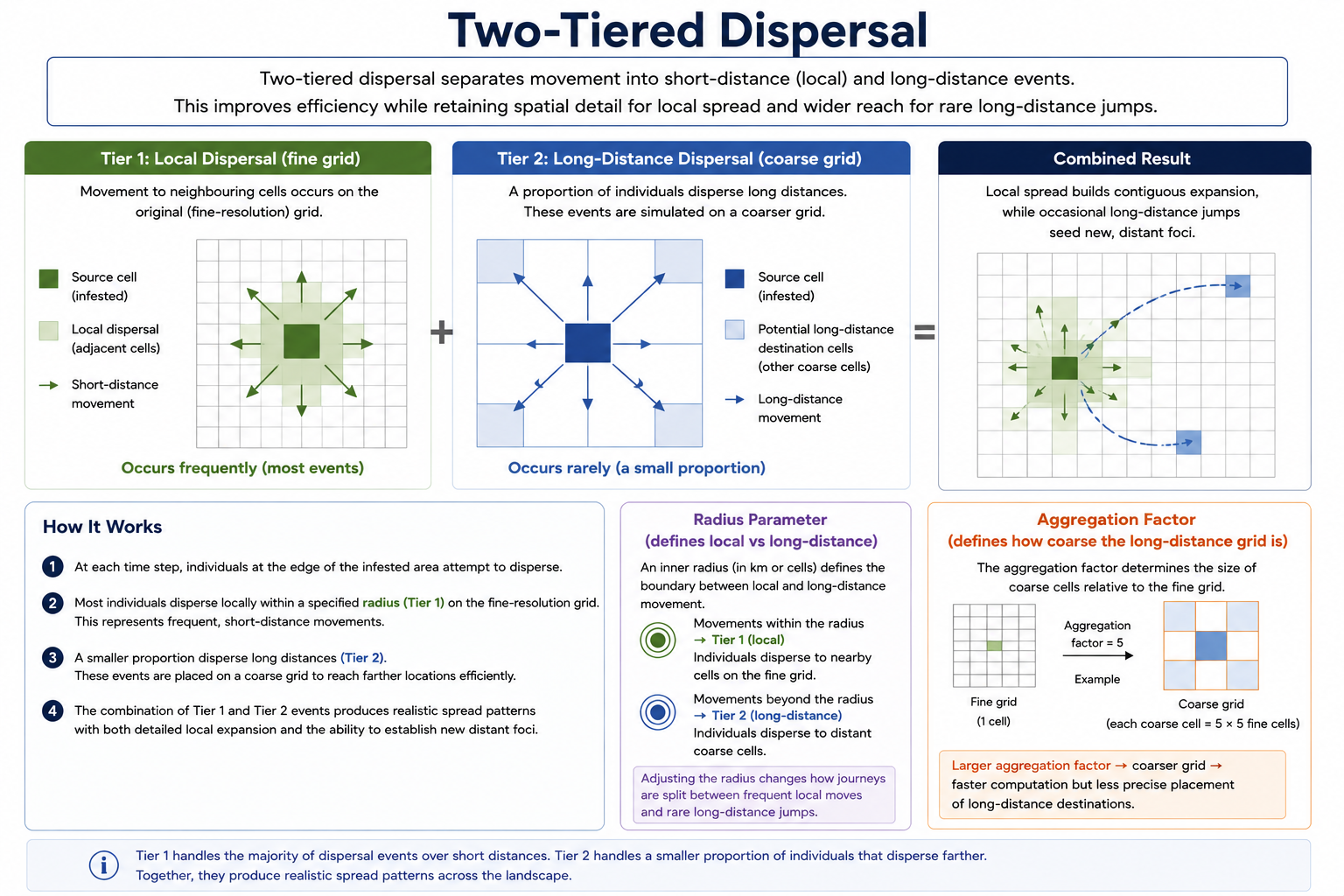
Two-tier Dispersal is a computational optimisation designed to improve the performance of large raster-based spread models while preserving a biologically appropriate raster resolution.

Rather than calculating all dispersal events at the original raster resolution, local dispersal is simulated on the original grid while long-distance dispersal is calculated on a temporary coarser grid before dispersers are redistributed back to the original raster. This substantially reduces computation time and memory requirements while retaining high spatial precision for local spread.

Two-tier Dispersal is controlled by two parameters:

• Inner Radius, which defines where the simulation transitions from the original raster resolution to the temporary aggregated grid; and
• Aggregation Factor, which determines the resolution of the temporary aggregated grid used for long-distance dispersal.

Importantly, neither parameter changes the underlying biological dispersal process. The distance organisms disperse remains entirely determined by the selected dispersal model. Instead, these parameters control how those calculations are performed computationally.

Inner Radius

Status: Required when Two-tier Dispersal is enabled

The Inner Radius defines the distance separating local and long-distance dispersal. Dispersal occurring within this distance is always simulated at the original raster resolution, whereas dispersal beyond the Inner Radius is calculated using the temporary aggregated grid before being redistributed back to the original study region resolution.

Although the Inner Radius is a computational parameter, its value should be informed by the biology of the species and the way local dispersal has been represented within the model. For most invasive species, the majority of dispersal occurs over relatively short distances, with only a small proportion of propagules dispersing much further. Because local dispersal determines the fine-scale pattern of invasion, it is generally desirable to simulate these movements at the full spatial resolution of the study region. In contrast, relatively infrequent long-distance dispersal events can usually be simulated on a coarser grid with little loss of biological realism while substantially improving computational performance.

When selecting an Inner Radius, consider the scale over which local spread is expected to occur and how this process has been parameterised within the chosen dispersal model. For example, if local spread is represented using a diffusion model or a dispersal kernel, the Inner Radius should generally encompass the distance over which most local dispersal events are expected to occur. This ensures that the dominant biological process governing local spread is simulated at the original raster resolution, while only relatively infrequent long-distance dispersal events utilise the aggregated grid.

Best practice

Select an Inner Radius that reflects the scale of the dominant local dispersal process rather than an arbitrary distance. For example, if a dispersal kernel indicates that most propagules disperse within approximately 20 km, an Inner Radius of around 20 km (or slightly greater) will ensure these biologically important local movements retain the full spatial resolution of the model. Larger values preserve more detail but reduce the computational benefits of two-tier dispersal, whereas smaller values increase computational efficiency but may reduce the spatial precision of local spread.

Aggregation Factor

Status: Required when Two-tier Dispersal is enabled

The Aggregation Factor controls the trade-off between computational efficiency and the spatial accuracy of long-distance dispersal. Larger Aggregation Factors improve computational performance by simulating long-distance dispersal on a coarser temporary grid, but they also reduce the spatial precision with which long-distance dispersal is represented.

The Aggregation Factor determines the resolution of the temporary aggregated grid used to simulate long-distance dispersal. For example, an Aggregation Factor of 5 applied to a study region with a 1 km raster resolution results in long-distance dispersal being simulated on a temporary 5 km grid before dispersers are redistributed back onto the original 1 km raster.

Best practice

Use the smallest Aggregation Factor that provides an acceptable improvement in computational performance. Very large Aggregation Factors should generally only be used for extremely large study regions where computational efficiency is a higher priority than fine-scale spatial accuracy. Whenever possible, the aggregated cell size should remain small relative to the characteristic distance of long-distance dispersal.

When should I use two-tier dispersal?

Network Model Configuration

Network models represent spread between discrete locations rather than across a continuous landscape. Consequently, the primary spatial configuration step is defining the locations (nodes) that comprise the network. Additional movement pathways and connection strengths are configured later when selecting a dispersal model.

Region Points

Status: Required

The Region Points define the locations (nodes) within the network. Each point represents a discrete location capable of supporting the target organism, such as a farm, orchard, nursery, port, warehouse, wetland or other management unit. Unlike raster models, where populations may establish in any grid cell, populations within a network model can establish and persist only at these predefined locations.

Best practice

Choose locations that represent biologically and operationally meaningful management units. The usefulness of the model depends on whether the selected nodes appropriately represent the system through which the organism spreads.

Spatially Implicit Model Configuration

Spatially implicit models do not explicitly represent geography and therefore require relatively little spatial configuration. The principal configuration option is defining the maximum area available for occupation during the simulation.

Maximum Implicit Area

Status: Optional

The Maximum Implicit Area defines the maximum area that can become occupied during the simulation. This parameter limits the potential extent of spread when modelling changes in occupied area through time.

If omitted, the model assumes there is no upper limit to the area that may become occupied, which may produce unrealistic estimates of invasion extent for some applications.

Best practice

Where possible, specify a biologically realistic maximum occupied area based on habitat availability, host distribution or the management region of interest.

Choosing a population model

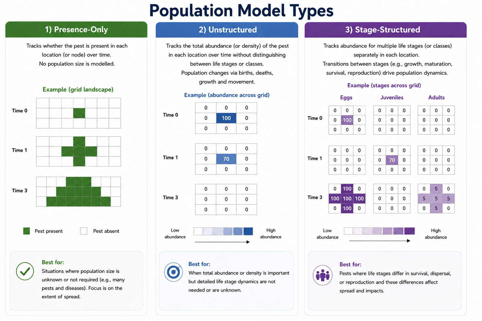
The population model defines how populations change through time following establishment. Although all population models can simulate the spread of an invasive species and determine which locations become occupied, they differ in how much biological detail is represented once a population has established.

Biosecurity Commons provides three population models of increasing biological complexity:

• Presence-only, which represents whether a location is occupied.
• Unstructured, which additionally models changes in total population abundance.
• Stage-structured, which further represents differences among life stages or age classes.

Choosing an appropriate population model is one of the most important biological decisions when constructing a spread model. More complex models can capture additional ecological processes, such as density-dependent population growth, carrying capacity and life-stage transitions, which may influence spread, impacts and management effectiveness. However, they also require substantially more biological information and introduce additional parameter uncertainty.

Consequently, the most appropriate population model is generally the simplest model capable of representing the biological processes expected to influence the management question.

Which population model should I choose?

Presence-only Population Model

The Presence-only model is the simplest population model available within Biosecurity Commons. Rather than representing the number of individuals present, each location is classified simply as occupied or unoccupied. Once a population establishes, the model tracks whether the location remains occupied and whether it can contribute to subsequent dispersal.

Because population abundance is not simulated, this model requires relatively few biological parameters and is particularly useful when abundance is difficult to estimate, biologically ambiguous, or unnecessary for addressing the management question (Jongejans et al. 2008; Bradhurst et al. 2021 ).

Recommended applications

• Plant diseases.
• Animal diseases.
• Early detection and preparedness.
• Spread forecasting where occupancy is the primary outcome.
• Situations where abundance data are unavailable.

Advantages

• Simple to parameterise. Requires relatively little biological information beyond establishment and dispersal processes.
• Computationally efficient. The absence of explicit population dynamics reduces simulation complexity.
• Well suited to many disease systems. For many pathogens, occupancy is easier to define than population abundance, making this model an appropriate representation of spread.
• Reduces parameter uncertainty. Fewer biological assumptions are required, reducing the likelihood of introducing poorly supported demographic parameters.

Limitations

• Does not represent changes in population abundance. Once established, all occupied locations are treated equally regardless of the number of individuals present.
• Cannot represent density-dependent processes. Population growth, carrying capacity and population regulation are not simulated.
• May oversimplify systems where abundance influences spread or impacts. If larger populations produce more propagules or greater impacts, a more detailed population model may be appropriate.

Although the Presence-only Population Model is the simplest of the three population models, it still allows users to represent two important biological processes: the probability that a dispersal event successfully establishes a new population, and any delay before that newly established population becomes capable of contributing to further spread.

Unstructured Population Model

The Unstructured Population Model represents changes in the total population abundance at each occupied location without distinguishing between life stages or age classes. Rather than tracking individual demographic processes, all individuals are assumed to contribute equally to population growth and dispersal (Jongejans et al. 2008).

Within Biosecurity Commons, population growth is governed by the finite population growth rate (λ), which defines how the total population changes between successive simulation time steps. A value of λ > 1 represents a growing population, λ = 1 represents a stable population, and λ < 1 represents a declining population.

The Unstructured Population Model provides a balance between biological realism and simplicity, making it suitable for many invasive species where total population abundance is expected to influence spread or impacts, but detailed demographic information is unavailable. It is often the preferred choice when occupancy alone is insufficient, but the additional complexity of modelling stage-specific population dynamics is not justified.

 Recommended applications

• Invasive plants.
• Environmental weeds.
• Invasive insects.
• Vertebrate pests.
• General population growth modelling.
• Situations where population abundance is expected to influence spread or impacts, but stage-specific demographic data are unavailable.

Advantages

• Represents changes in population abundance. Population size can increase or decrease through time rather than simply recording whether a location is occupied.
• Accounts for density-dependent population growth. Carrying capacity can limit population growth, allowing populations to stabilise as resources become limiting.
• Flexible population growth. The finite population growth rate (λ) can be specified as a constant or allowed to vary through space, time, or both, enabling the model to represent environmental heterogeneity, seasonal population dynamics and changing management conditions.
• Requires relatively few biological parameters. Compared with a Stage-structured Population Model, relatively little demographic information is required while still providing substantially greater biological realism than a Presence-only model.
• Suitable for many invasive species. Provides an effective balance between biological realism, computational efficiency and parameter requirements for species where total abundance influences invasion dynamics.

Limitations

• Assumes all individuals are demographically equivalent. Differences in survival, reproduction and dispersal among life stages or age classes are not represented.
• May oversimplify species with complex life histories. Species with distinct juvenile and adult stages, delayed maturation or stage-specific reproduction may require a Stage-structured Population Model.
• Requires estimates of population growth. Reliable estimates of the finite population growth rate (λ), and where appropriate carrying capacity, may not always be available, particularly for newly emerging invasive species.
• Cannot represent stage-specific management. Management actions targeting particular life stages or age classes cannot be explicitly modelled.

Stage-structured Population Model

The Stage-structured Population Model explicitly represents different life stages or age classes within the population (Leslie, 1945; Lefkovitch, 1965). Population dynamics are governed by stage-specific survival, reproduction and transitions between stages, allowing the model to capture demographic processes that cannot be represented using a single overall population growth rate.

Unlike the Unstructured Population Model, different life stages may also be assigned different biological characteristics. This provides greater flexibility when modelling species for which dispersal, impacts or management effectiveness differ among life stages. For example, juvenile stages may disperse differently from adults, only reproductive adults may contribute to population growth, or management actions may target specific life stages such as eggs, larvae or adults.

Stage-structured models are commonly informed by life table analyses or stage-transition matrices, particularly for insects and other organisms with well-defined developmental stages. These data describe stage-specific survival, development and reproduction, allowing the model to represent the life cycle explicitly.

This is the most biologically realistic population model available within Biosecurity Commons and is most appropriate when life-history characteristics are expected to influence spread, impacts or management effectiveness.

Recommended applications

• Forest pests.
• Long-lived plants.
• Invasive insects with distinct developmental stages.
• Species with well-defined life histories informed by life table analyses.
• Management strategies targeting specific life stages.
• Species with well-understood demographic data.

Advantages

• Represents demographic structure explicitly. Survival, reproduction and transitions can differ among life stages.
• Supports stage-specific dispersal. Different life stages can contribute differently to spread, allowing the model to better represent species where dispersal behaviour changes throughout the life cycle.
• Supports stage-specific impacts. Different life stages may contribute differently to economic, environmental or social impacts.
• Supports stage-specific management. Management actions targeting particular life stages can be represented explicitly, allowing alternative intervention strategies to be evaluated.
• Provides the greatest biological realism. Complex life histories, delayed maturation and stage-dependent reproduction can be represented naturally.

Limitations

• Requires substantially more biological information. Stage-specific survival, reproduction and transition parameters are often unavailable for invasive species, particularly during preparedness or the early stages of an incursion.
• Often requires life table or demographic data. Reliable parameterisation typically depends on published life tables, transition matrices or experimental studies describing the species' life history.
• Greater parameter uncertainty. Additional parameters increase the potential for uncertainty to influence model predictions.
• More complex to parameterise and interpret. Constructing an appropriate stage-transition model requires a good understanding of the species' biology and life history.
• Additional complexity does not necessarily improve predictions. If stage-specific processes have little influence on the management question, simpler population models may provide equally robust and more transparent predictions.

Configure Population Parameters

Once a population model has been selected, the next step is to configure the parameters governing establishment, population growth and demographic processes. The available parameters depend on the selected population model. Simpler models require relatively few parameters, whereas more biologically realistic models require additional demographic information.

Several parameters are common across multiple population models, while others are unique to a particular modelling approach. Biosecurity Commons also provides optional modifiers that allow population dynamics to vary across space, through time, or both, enabling users to represent environmental heterogeneity, seasonal dynamics and changing management conditions.

Parameter Availability Summary

Threat Suitability

Status: Required (Raster and Network models only)

Applies to:

• Presence-only
• Unstructured
• Stage-structured

Available inputs:

• Raster (spatial or spatio-temporal)
• Point dataset (Network models)

Threat Suitability defines the probability that a dispersal event successfully establishes a new population after arriving at a location. It links the dispersal and establishment processes by determining whether arriving propagules successfully form a persistent population. Values range between 0 and 1, where larger values indicate a greater likelihood of successful establishment.

In most applications, Threat Suitability is derived from the Establishment Likelihood workflow, allowing establishment probability to vary across space and, where appropriate, through time according to changes in environmental suitability. Alternatively, users may supply an independently derived suitability layer.

Threat Suitability may be specified as either a single static layer or a time-varying series of suitability layers. When using time-varying data, each layer should correspond to one simulation time step (for example, monthly suitability layers for a model using monthly time steps). If the simulation contains more time steps than the number of supplied suitability layers, Biosecurity Commons assumes the layers represent a repeating cycle and automatically reuses them in the order provided. For example, a set of 12 monthly suitability layers will be repeated each year in a multi-year simulation.

Common mistake

Threat suitability is not the same as the Establishment Likelihood generated by the Establishment Likelihood workflow. Establishment Likelihood estimates the probability of an initial establishment event by combining the spatial distribution of introduction pathways (arrival risk) with the probability that that the environment is suitable for establishment. It is therefore primarily used to identify where new incursions are most likely to occur and can be used to inform the random seeding of initial introductions in spread simulations.

Threat suitability, in contrast, represents only the relative suitability of local environmental conditions for establishment following a spread event. It does not account for introduction pathways or arrival risk. Instead, it determines the probability that dispersing individuals successfully establish after reaching a location and therefore influences the spread dynamics of an existing population.

Best practice

Where possible, derive Threat Suitability from the Establishment Likelihood workflow rather than assuming a constant establishment probability across the study region.

Spread Delay

Status: Optional

Applies to:

• Presence-only

Available inputs

• Single value (simulation time steps)

Spread Delay specifies the number of simulation time steps that must elapse between successful establishment and the ability of that population to contribute to further spread. During this period, the population is considered established but does not generate dispersers.

Spread Delay represents biological processes that occur between establishment and the onset of dispersal. Depending on the species, this may correspond to maturation, population build-up or latent infection periods. For example, an invasive tree may require many years before producing seed, whereas many pathogens or insect pests may become capable of dispersing within a single simulation time step.

Best practice

Choose a Spread Delay that reflects the biology of the target organism and ensure it is interpreted relative to the selected simulation time step.

Finite Population Growth Rate (λ)

Status: Required

Applies to:

• Unstructured

Available inputs:

• Single value
• Spatial only
• Temporal only
• Spatio-temporal

The Finite Population Growth Rate (λ) defines the multiplicative change in population abundance between successive simulation time steps. For example, λ = 1.2 indicates that the population increases by approximately 20% per time step, whereas λ = 1 represents a stable population and values below 1 represent population decline.

Within Biosecurity Commons, λ may be supplied in four ways:

• Single value — applies the same growth rate across all locations and simulation time steps.
• Spatial only — allows growth rates to vary among locations while remaining constant through time. For raster models, this is supplied as a raster layer; for network models, it is supplied as a point-based CSV.
• Temporal only — allows growth rates to vary between simulation time steps while remaining uniform across the study region. This is supplied as a temporal CSV series and may be used to represent seasonality, interannual variation or other time-dependent processes.
• Spatio-temporal — allows growth rates to vary across both locations and time. For raster models, this is supplied as a multilayer raster; for network models, it is supplied as a CSV containing sequential growth columns.

Where a Carrying Capacity is specified, realised population growth slows as abundance approaches the local carrying capacity.

Best practice

Choose the simplest input type that adequately represents the available biological evidence. Use spatial, temporal or spatio-temporal growth inputs only where there is a defensible basis for the variation represented.

Ensure that any temporal or spatio-temporal growth data correspond to the simulation time step. For example, monthly growth inputs should be used with monthly simulation steps.

Carrying Capacity (K)

Status: Optional

Applies to:

• Unstructured
• Stage-structured

Available inputs:

Raster and Network models

• Spatial only
• Spatio-temporal

Spatially Implicit models

• Single value
• Temporal

Carrying Capacity (K) defines the maximum sustainable population size at a location or per unit area. As population abundance approaches this limit, density-dependent regulation reduces population growth, preventing the population from increasing indefinitely (Ricker, 1958).

For Raster and Network models, carrying capacity is specified separately for each location:

• Spatial only applies a static carrying capacity throughout the simulation. Raster models use a single raster layer, while Network models use a point-based CSV containing a capacity value for each location.
• Spatio-temporal allows carrying capacity to vary among locations and through time. Raster models use a multilayer raster containing sequential temporal layers, while Network models use sequential columns such as capacity_1, capacity_2, and so forth.

For Spatially Implicit models, carrying capacity is specified per unit area:

• Single value applies a constant carrying capacity throughout the simulation.
• Temporal allows carrying capacity to vary through time using a CSV time series.

When carrying capacity is configured for a Spatially Implicit model, users must also specify the Capacity Area Unit:

• metres squared;
• kilometres squared; or
• maximum area, where a Maximum Implicit Area has been defined.

Important Note: If a maximum occupied area is specified, the model converts the total carrying capacity into a carrying capacity per unit area. For example, if the carrying capacity is 10,000 individuals and the maximum area is 100 km², the resulting carrying-capacity density is 100 individuals per km². This density is then used to relate population abundance to the area occupied.

If the number of supplied temporal layers, columns or rows is shorter than the number of simulation time steps, Biosecurity Commons treats the values as a repeating cycle. For example, 12 monthly carrying-capacity values will be repeated annually in a multi-year simulation.

Carrying capacity may also be configured as dynamically impacted by the incursion. This links capacity to dynamic impacts specified later in the Impacts section, allowing the invading population to progressively reduce the availability of a resource or asset on which it depends.

Best practice

Use spatially or temporally varying carrying capacity only where there is a defensible ecological basis for that variation. Carrying capacity may be informed by host density, habitat extent, food availability or another limiting resource.

Where a suitability layer is used to derive carrying capacity, document the assumed relationship. For example, users may assume that a location with a suitability score of 0.5 supports half the population of a location with a suitability score of 1, but Biosecurity Commons does not impose this relationship automatically.

Ensure that temporal carrying-capacity inputs correspond to the selected simulation time step. For example, monthly capacity data should be used with monthly simulation steps.

Transition Matrix

Status: Required

Applies to:

• Stage-structured

Available inputs:

• Stage/Age-transition matrix

The Transition Matrix defines how individuals survive, reproduce and transition between life stages (Lefkovitch, 1965) or ages (Leslie, 1945) during each simulation time step. Each element of the matrix specifies either the probability of surviving and remaining within a stage/age, surviving and progressing to another stage/age, or contributing new individuals through reproduction.

Unlike the Unstructured Population Model, which summarises population growth using a single finite population growth rate (λ), the Transition Matrix explicitly represents the demographic processes responsible for population growth. This allows different life stages to contribute differently to reproduction, dispersal, impacts and management, providing a much more flexible representation of species with complex life histories.

At each simulation time step, the Transition Matrix is multiplied by the current population vector to calculate the abundance of each life stage in the following time step.

How does a Transition Matrix work?

Rows represent the life stage after one simulation time step, while columns represent the life stage at the current simulation time step. Each column therefore describes what happens to individuals currently occupying that life stage.

For example, consider an insect with four life stages:

• Egg
• Larva
• Pupa
• Adult

A simplified Transition Matrix may be:

This matrix can be interpreted as follows:

• Each reproductive adult produces an average of 25 new eggs during one simulation time step.
• 70% of eggs survive and develop into larvae.
• 20% of larvae remain in the larval stage for another time step.
• 75% of larvae develop into pupae.
• 30% of pupae remain in the pupal stage.
• 65% of pupae develop into adults.
• 90% of adults survive and remain adults between successive time steps.

The resulting population vector is then used as the starting population for the next simulation time step, and the process is repeated throughout the simulation.

Additional modelling considerations

When constructing a Transition Matrix, several additional considerations are important to ensure the model accurately represents the biology of the target species.

Simulation time step

The Transition Matrix should correspond to the simulation time step used by the model. For example, weekly simulations require weekly transition probabilities, whereas annual simulations require annual transition probabilities. If published life table data are reported at a different temporal resolution, the transition probabilities should be converted accordingly before being incorporated into the model.

Sex ratio and fecundity

Many published life tables and demographic matrices, particularly for insects, are constructed using female-only populations because females determine the reproductive output of the population. When parameterising a Stage-structured Population Model, users should carefully consider whether the simulated population represents:

• females only;
• males and females combined; or
• another subset of the population.

If modelling both sexes, fecundity values should be adjusted to account for the assumed sex ratio unless this has already been incorporated into the published demographic data. Failure to do so may substantially overestimate or underestimate population growth.

Stage definitions

Each life stage should represent a biologically meaningful developmental stage (for example, egg, larva, pupa and adult) or age class. The number of stages should be sufficient to capture important differences in survival, reproduction, dispersal or management without introducing unnecessary complexity.

Where supported by Biosecurity Commons, stage-specific dispersal, impacts and management actions may also be assigned to individual life stages, allowing users to represent processes such as highly mobile adults, sedentary juvenile stages, or management strategies targeting specific stages of the life cycle.

Parameter sources

Transition matrices are commonly derived from:

• published life table analyses;
• demographic studies;
• laboratory or field experiments;
• published Leslie or Lefkovitch matrices; and
• expert elicitation where empirical data are unavailable.

For many invasive insects, published life table analyses provide the most appropriate basis for estimating stage-specific survival and fecundity.

Best practice

Construct the Transition Matrix using published life table analyses or demographic studies wherever possible, ensuring that transition probabilities and reproductive rates correspond to the selected simulation time step. Keep the matrix as simple as possible while still representing the biological processes expected to influence spread, impacts or management decisions.

Growth Variation

Status: Optional

Applies to

• Stage-structured Population Model

Available configuration

Demographic process

• Reproduction
• Survival
• Both reproduction and survival

Life stages

• All stages
• Selected stages

Variation

• Spatial
• Temporal
• Spatio-temporal

Growth Variation provide additional flexibility by allowing the demographic rates defined by the Transition Matrix to vary across space, through time, or both. Rather than replacing the underlying demographic model, Growth Variation applies multiplicative modifiers that reduce survival, reproduction, or both in response to environmental conditions, seasonal variation or management interventions.

When using a Growth variation, the Transition Matrix should represent the species under optimal (or most favourable) conditions. Growth Variation then defines the proportion of this demographic potential that is realised throughout the simulation.

Growth Variation allows demographic rates within the Transition Matrix to vary according to environmental conditions, seasonal dynamics or management interventions. Rather than requiring users to construct multiple Transition Matrices, Growth Variation applies multiplicative modifiers to the existing matrix during the simulation.

Growth Variation values range between 0 and 1, where:

• 1.0 represents optimal conditions and no reduction in demographic performance.
• 0.8 represents 80% of the baseline demographic rate.
• 0.5 represents 50% of the baseline demographic rate.
• 0.0 completely inhibits the selected demographic process.

When configuring Growth Variation, users specify:

• which demographic process is modified (reproduction, survival, or both);
• which life stage(s) the modifier applies to (all stages or selected stages); and
• how the modifier varies (spatially, temporally, or both).

This provides considerable flexibility when representing species whose demographic processes respond differently to changing environmental conditions or management actions.

How does Growth Variation work?

Growth Variation multiplies the selected demographic rates within the Transition Matrix by the specified modifier.

For example, suppose the Transition Matrix represents an insect population under optimal environmental conditions.

Example 1 – Modifying reproduction

If each adult female produces 25 eggs per simulation time step under optimal conditions, applying a reproduction modifier reduces fecundity while leaving survival unchanged.

This option is useful for representing processes such as:

• seasonal breeding;
• drought reducing egg production;
• host quality affecting fecundity; or
• management actions that reduce reproduction.

Example 2 – Modifying survival

If larval survival under optimal conditions is 0.70, applying a survival modifier changes the realised survival probability while leaving reproduction unchanged.

This option is useful for representing:

• overwinter mortality;
• pesticide applications;
• disease;
• drought-induced mortality; or
• changes in host quality affecting survival.

Example 3 – Applying Growth Variation to selected life stages

Growth Variation may be applied to all life stages or restricted to selected stages.

For example, suppose a pesticide targets only larvae. A survival modifier of 0.5 could be applied to the larval stage while all other life stages remain unaffected.

In this example, larval survival is reduced by 50%, whereas survival of eggs, pupae and adults remains unchanged.

Similarly, Growth Variation could be applied only to adult reproduction, allowing seasonal breeding or environmental conditions to influence fecundity without affecting juvenile development or adult survival.

Example 4 – Modifying both reproduction and survival

When Both is selected, Growth Variation is applied simultaneously to the fecundity and survival components of the Transition Matrix.

This effectively scales the realised demographic performance represented by the Transition Matrix while preserving its underlying demographic structure. It is appropriate where environmental conditions or management actions broadly influence overall population performance rather than a single demographic process.

Configuration options

Spatial

Growth Variation is supplied as a spatial dataset, allowing demographic performance to vary among locations according to environmental conditions, habitat quality or resource availability.

Temporal

Growth Variation is supplied as a temporal series, allowing demographic performance to vary between simulation time steps. This is useful for representing seasonal population dynamics, annual climatic variation or changing management conditions.

Spatio-temporal

Growth Variation varies across both space and time, allowing environmental conditions and seasonal processes to interact. This provides the greatest flexibility and is particularly useful where temporal dynamics differ among locations.

When temporal or spatio-temporal Growth Variation is used, each temporal layer or record should correspond to a single simulation time step. If fewer temporal layers are supplied than simulation time steps, Biosecurity Commons assumes the values represent a repeating cycle and applies them sequentially throughout the simulation.

Best practice

Construct the Transition Matrix using demographic rates measured under optimal or most favourable conditions. Growth Variation should then be used to represent reductions in demographic performance resulting from environmental conditions, seasonal processes or management interventions.

Apply Growth Variation only to the demographic processes and life stages expected to vary. For example, drought may primarily reduce reproduction, whereas pesticide application may primarily reduce larval survival.

Use the simplest Growth Variation required to represent the biology of the species. For many applications, a single temporal or spatial modifier will be sufficient.

Initialisation

Initialisation defines the starting conditions of the simulation by specifying where the invasion begins and the characteristics of the initial population. Because spread models simulate invasions forward through time, the choice of initialisation can strongly influence the subsequent pattern and timing of spread, particularly during the early stages of an invasion.

The most appropriate initialisation method depends on the management question being addressed. When modelling a known incursion, the initial population is typically specified using observed infestation data. Conversely, preparedness and sensitivity analyses often require hypothetical incursions to be introduced at uncertain locations.

For raster and network models, Biosecurity Commons provides two methods for defining the initial distribution of the population:

• Initial Layer, where the initial population is explicitly specified.
• Random Location, where one or more introduction locations are generated probabilistically.

For spatially implicit models, geography is not represented explicitly, so users specify only the initial population size.

Which initialisation method should I choose?

Initial Layer

The Initial layer defines the spatial distribution of the invasive species at the beginning of the simulation.

The initial population may be specified as either a population count (i.e. for unstructured and stage-structured population models) or presence-only (i.e. presence-only population models) dataset. Population count inputs define the initial abundance at each raster cell or network node, whereas presence-only inputs indicate whether the species is initially present or absent.

For raster models, the initial distribution may be supplied as a raster layer or created interactively by drawing one or more introduction points or occupied areas.
Note: When using the drawing capability users will be prompted to specify a population size which will be uniformly distributed across the selected area.

For network models, the initial population is specified using a CSV associated with each network node.

Recommended applications

• Known infestations.
• Delimitation and response modelling.
• Forecasting the spread of an existing invasion.
• Evaluating specific introduction scenarios.

Advantages

• Represents known starting conditions.
• Fully reproducible between simulation runs.
• Allows complex initial distributions to be represented.

Limitations

• Requires knowledge of the initial infestation.
• Does not account for uncertainty in the introduction location.

Random Location

The Random Location method generates an initial incursion probabilistically. Rather than specifying exactly where an invasion begins, users provide a spatial weighting layer describing the relative likelihood of introduction. For each simulation replicate, one introduction location is randomly sampled from this distribution, meaning different simulations may begin in different locations.

For raster models, the weighting layer is supplied as a raster, while network models use a CSV containing a relative weighting for each node.

In many applications, the weighting layer is derived from the Establishment Likelihood workflow. This allows introduction locations to be sampled according to the estimated likelihood of successful establishment, ensuring that incursions are more likely to occur in environmentally suitable areas while still accounting for uncertainty in the precise location of introduction. Alternatively, users may supply any other spatial weighting layer representing the relative likelihood of introduction, such as pathway-specific arrival risk or expert-derived introduction probabilities.

Because each simulation may begin in a different location, Random Location is particularly useful for preparedness planning, sensitivity analyses, and evaluating surveillance or management strategies when the exact location of a future incursion is unknown.

Recommended applications

• Preparedness planning.
• Border surveillance.
• Pathway analysis.
• Sensitivity analysis.
• Multiple incursion scenarios.

Advantages

• Represents uncertainty in introduction locations.
• Allows stochastic introduction scenarios.
• Well suited to repeated simulation experiments.

Limitations

• Requires relative introduction weights.
• Individual simulation replicates may differ substantially depending on the sampled incursion location.

Initial Age

Status: Optional

Applies to:

• Presence-only
• Stage-structured

Initial Age specifies the age of the initial population, measured in simulation time steps.

For the Presence-only Population Model, Initial Age offsets the remaining Spread Delay, allowing simulations to begin with populations that have already partially matured and may therefore begin contributing to dispersal sooner.

For the Stage-structured Population Model, Initial Age determines the demographic composition of the initial population. Using the specified Transition Matrix, Biosecurity Commons estimates the expected distribution of individuals among the defined life stages (for example, eggs, larvae, pupae and adults) for a population of the specified age. This allows simulations to begin with a biologically realistic stage structure rather than assuming all individuals occupy the same life stage.

Initial Age may be specified as either:

• a single value applied to all initial populations; or
• a spatial layer allowing the initial age to vary among introduction locations.

When Initial Age is provided, the stage composition of the initial population is derived automatically from the Transition Matrix.

Best practice

Specify Initial Age whenever information is available on how long the initial population has been established prior to the start of the simulation. Ensure that age is interpreted relative to the selected simulation time step.

First Occupancy Stages

Status: Required (when Initial Age is not specified)

Applies to:

• Stage-structured Population Model
• Initial Layer only

First Occupancy Stages specifies which life-stages/ages are present at first occupancy. If (and where) the initial age is specified, first occupancy is assumed to occur prior to the beginning of model simulations (when age = 0), otherwise first occupancy coincides with the beginning of model simulations. If initial age is specified, the composition of life-stages/ages at the beginning of model simulations is adjusted appropriately, whereby the stage/age composition is projected forward from first occupancy (at age = 0) via stage/age matrix. A checkbox will appear for each stage/age (i.e. column) specified in the growth matrix for users to select. If none are selected, all stages are assumed to be applicable.

Incursion Mean

Status: Required

Applies to:

• Random Location initialisation type
• Unstructured Population Model
• Stage-structured Population Model

Incursion Mean defines the expected founder population size for each randomly generated introduction. The realised population size is sampled from a Poisson distribution with the specified mean for each simulation replicate.

Best practice

Choose a mean founder population consistent with the likely propagule size associated with the introduction pathway.

Incursion Stages

Status: Required

Applies to:

• Random Location initialisation type
• Stage-structured Population Model

Incursion Stages specify which life stages may be present following a randomly generated introduction. Users select one or more stages from those defined within the Transition Matrix. If no stages are selected, all stages are assumed to be possible.

Best practice

Select only those life stages consistent with the pathway being represented.

Choosing a Dispersal Model

Dispersal determines how organisms move from occupied locations and establish new populations elsewhere. Together with population growth and establishment, dispersal governs the rate, direction and spatial pattern of biological invasions, making it one of the most influential processes in spread modelling.

The most appropriate dispersal model depends on the biology of the species, the dominant dispersal mechanisms, the selected spatial framework, and the management question being addressed. Some organisms spread gradually through local diffusion, whereas others disperse via infrequent long-distance movements or well-defined transport pathways (Wilson et al. 2009; Gippet et al. 2019).

The available dispersal functions within Biosecurity Commons depend on both the selected Spatial Framework and Population Model. Raster and Network models explicitly represent movement across landscapes or networks and therefore allow multiple dispersal functions to be combined within a single simulation. This enables users to represent multiple dispersal pathways simultaneously, such as natural spread together with human-assisted transport.

In contrast, Spatially Implicit models do not explicitly represent geography. Instead, they describe changes in the overall occupied area or population size through time and therefore provide specialised dispersal functions that model how occupied area expands rather than where organisms move.

Which dispersal models are available?

For Raster and Network models, multiple dispersal functions may be added to represent different dispersal mechanisms or pathways. For example, local spread may be represented using Diffusion, while rare long-distance dispersal is represented using one or more Kernel Dispersal functions.

Which dispersal model should I choose?

Many invasive species spread through multiple mechanisms operating simultaneously. For example, an insect may disperse locally through natural flight while also being transported over long distances by vehicles. In these situations, Raster and Network models can combine multiple dispersal functions within a single simulation to represent each dispersal pathway independently.

Kernel Dispersal

Kernel Dispersal models the movement of individuals or propagules by drawing dispersal distances from a probability distribution (a dispersal kernel). Each dispersal event is independent, allowing most movements to occur over relatively short distances while still representing occasional long-distance dispersal events.

The shape of the kernel determines how rapidly dispersal probability declines with distance and therefore controls the balance between local and long-distance spread. Different kernel functions can represent a wide variety of dispersal mechanisms, from highly localised seed dispersal to infrequent human-assisted movement.

Kernel Dispersal is available for both Raster and Network models and may be combined with other dispersal functions within the same simulation.

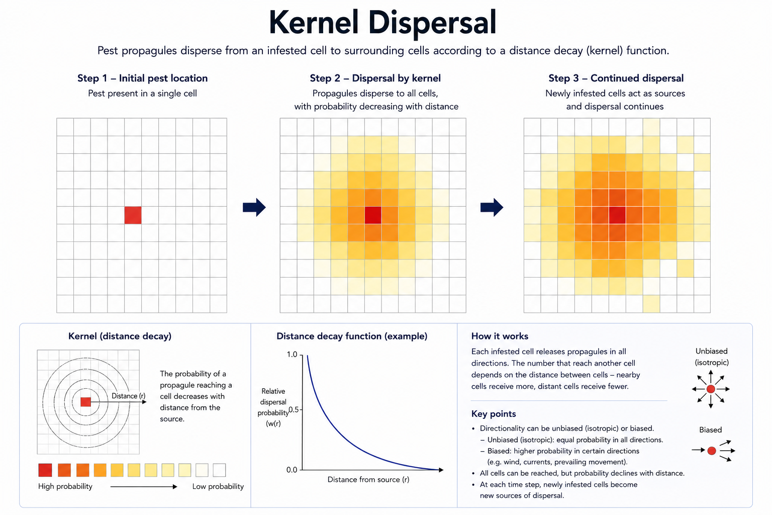
Recommended applications

• Flying insects
• Seed dispersal
• Wind dispersal
• Animal movement
• Human-assisted spread
• Rare long-distance dispersal events

Advantages

• Represents stochastic dispersal naturally.
• Can represent both short- and long-distance dispersal.
• Supports numerous dispersal-distance functions.
• Multiple kernel functions may be combined to represent different pathways.
• Easily incorporates landscape modifiers such as attractors, permeability and directional bias.

Limitations

• Requires assumptions about dispersal-distance distributions.
• Long-distance spread can be sensitive to kernel selection.
• Reliable dispersal-distance data are often unavailable.

Dispersal Diffusion

Dispersal Diffusion represents spread as gradual expansion from occupied locations across a continuous raster landscape. Rather than modelling individual long-distance dispersal events, diffusion assumes populations spread primarily through repeated local movements, producing a relatively continuous invasion front.

This approach is most appropriate where spread is dominated by neighbouring populations progressively colonising adjacent areas. Landscape modifiers such as directional spread, attractors and permeability may be incorporated to allow diffusion rates to vary across the landscape.

Dispersal Diffusion is available only for Raster models.

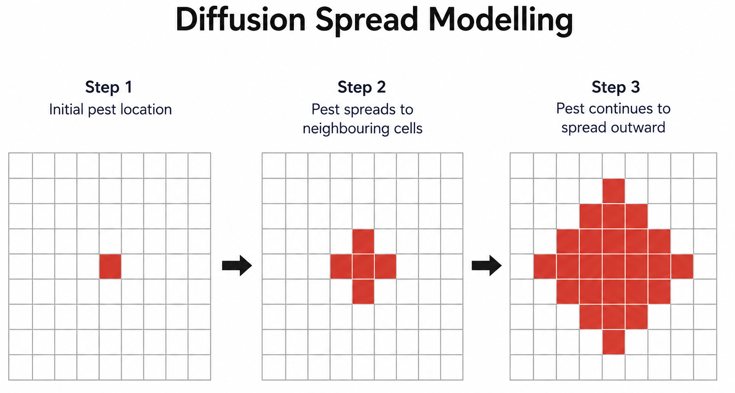
Recommended applications

• Environmental weeds
• Plant diseases
• Soil-borne organisms
• Slowly expanding invasions
• Continuous invasion fronts

Advantages

• Represents local spread intuitively.
• Requires relatively few parameters.
• Produces realistic invasion fronts.
• Can incorporate landscape heterogeneity.

Limitations

• Does not naturally represent rare long-distance dispersal.
• May underestimate human-assisted movement.
• Restricted to Raster models.

Dispersal Gravity

Dispersal Gravity represents movement between known locations as a function of both the attractiveness of destination nodes and the distance separating them. Larger or more attractive destinations receive more dispersers, while movement generally declines with increasing distance.

Gravity models are particularly well suited to pathway-based movement where organisms disperse through transport, trade or other well-defined movement networks rather than continuously across a landscape.

Dispersal Gravity is available only for Network models.

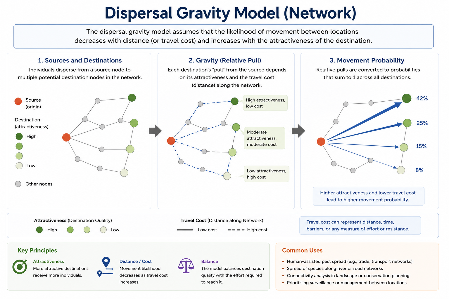
Recommended applications

• Livestock movement
• Freight transport
• Nursery trade
• Commodity movement
• Transport networks
• Human-assisted spread

Advantages

• Explicitly represents movement between known locations.
• Incorporates destination attractiveness.
• Accounts for distance decay.
• Well suited to pathway-based dispersal.

Limitations

• Requires estimates of movement between nodes.
• Requires estimates of destination attractiveness.
• Does not represent continuous landscape diffusion.
• Restricted to Network models.

Radial Diffusion

Radial Diffusion is the dispersal function available for Presence-only Spatially Implicit models. Rather than explicitly modelling movement across a landscape, it assumes the occupied area expands outward at a constant radial rate through time.

Because geography is not represented explicitly, Radial Diffusion predicts changes in the total occupied area rather than the spatial pattern of spread. It is therefore most appropriate when the objective is to estimate overall rates of spread rather than identify where spread occurs.

Recommended applications

• Presence-only population models
• Rapid exploratory analyses
• Broad-scale spread estimates
• Homogeneous landscapes

Advantages

• Extremely simple to parameterise.
• Computationally efficient.
• Requires only an average radial spread rate.

Limitations

• Available only for Presence-only Spatially Implicit models.
• Assumes homogeneous landscapes.
• Does not predict where spread occurs.
• Cannot represent abundance-dependent spread.

Area Spread

Area Spread is available for Unstructured and Stage-structured Spatially Implicit models. It assumes the occupied area increases directly in proportion to population abundance. Consequently, no additional dispersal parameters are required because changes in occupied area are determined entirely by the underlying population dynamics.

This approach provides a simple relationship between population growth and occupied area and is appropriate when explicit modelling of dispersal is unnecessary.

Recommended applications

• Simple abundance-based spread models
• Benefit-cost analyses
• Exploratory scenario analyses
• Situations where occupied area closely follows population size

Advantages

• No dispersal-specific parameters.
• Computationally efficient.
• Simple relationship between abundance and occupied area.

Limitations

• Assumes occupied area is proportional to abundance.
• Does not explicitly model dispersal.
• Does not predict where spread occurs.

Reaction-Diffusion

Reaction-Diffusion is available for Unstructured and Stage-structured Spatially Implicit models. It represents spread as the interaction between:

• Reaction — changes in population abundance through population growth and demographic processes; and
• Diffusion — spatial expansion of the population from its point of introduction.

Rather than prescribing occupied area directly, Reaction-Diffusion calculates the radius of the occupied area from the change in population abundance through time and the specified diffusion rate or diffusion coefficient. As the population grows, the occupied area expands radially. When population growth slows, for example as abundance approaches carrying capacity, the rate of spatial expansion also slows.

This differs from Area Spread, where occupied area is derived directly from population abundance relative to the population's carrying capacity per unit area. Reaction-Diffusion instead represents an expanding invasion front in which demographic growth and diffusion jointly determine the rate of spatial expansion.

By default, the occupied area may also contract if population abundance declines, although contraction can be disabled where a declining population is expected to persist across its previously occupied range.

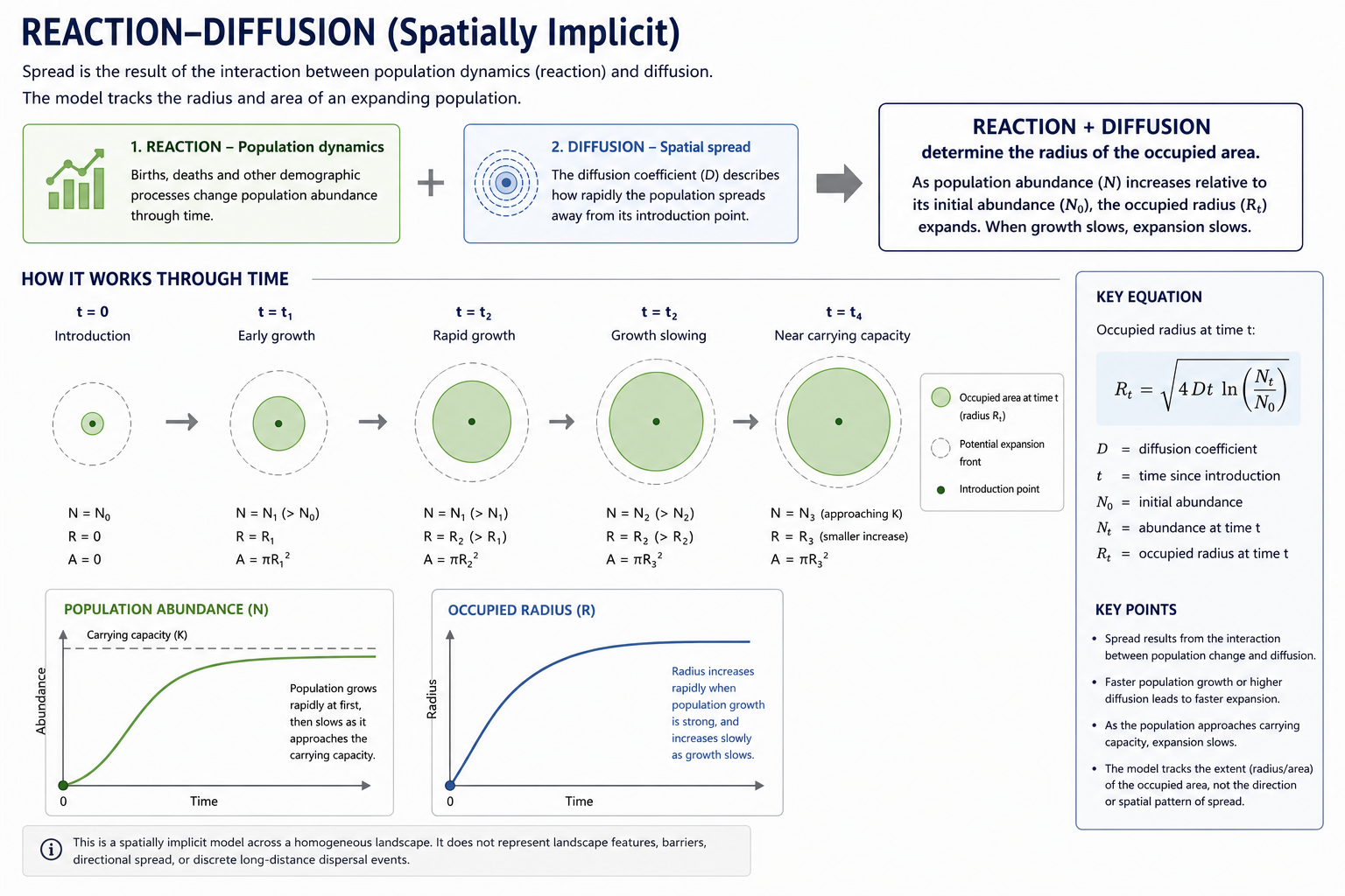
Recommended applications

• Spatially implicit invasions where local spread can reasonably be approximated as radial diffusion.
• Populations where both demographic growth and dispersal influence the rate of range expansion.
• Invasions where spread is expected to slow as population growth becomes constrained by carrying capacity.
• Analyses requiring a mechanistic relationship between population abundance and spatial expansion without explicitly modelling the landscape.

Advantages

• Links population dynamics directly to the rate of spatial expansion.
• Represents the interaction between demographic growth and diffusive spread.
• Naturally allows spread to slow as population growth becomes constrained.
• Can represent contraction of the occupied area following population decline.
• Computationally efficient because the spatial distribution is represented implicitly rather than as individual grid cells.

Limitations

• Available only for Unstructured and Stage-structured Spatially Implicit models.
• Assumes radial spread across a spatially homogeneous landscape.
• Represents the extent of the occupied area but not the geographical direction or spatial pattern of spread.
• Does not represent landscape heterogeneity, barriers, directional spread or discrete long-distance dispersal.
• Requires a diffusion rate in addition to the parameters governing population dynamics.

Configure Dispersal Functions

Once one or more dispersal functions have been added to the model, the next step is to configure how populations spread throughout the simulation. These parameters determine how dispersers are generated, how they move through the landscape, and how additional biological or environmental processes influence the realised pattern of spread.

The available parameters depend on the Spatial Framework, Population Model and Dispersal Function selected earlier in the workflow. For example, Raster and Network models support different dispersal functions and landscape modifiers, while Presence-only and abundance-based population models use different approaches to generate dispersers. Consequently, only the parameters relevant to the selected modelling framework are displayed.

Dispersal can generally be configured in three stages:

1. Generate Dispersers – Determines how many dispersal events or dispersing individuals are generated during each simulation time step.
2. Define the Dispersal Process – Specifies how dispersers move using the selected dispersal function. Depending on the chosen model, this may involve configuring a distance kernel, diffusion process, gravity model or other movement process.
3. Modify Dispersal – Optionally modifies the underlying dispersal process to account for additional biological, environmental or computational processes, such as habitat attractiveness, landscape permeability, directional spread or two-tier dispersal.

Although these stages are configured separately, they operate sequentially within the simulation. The Population Model first determines how many dispersers are available, the selected Dispersal Function determines how those dispersers move, and any optional modifiers then adjust the realised pattern of spread before arriving propagules are evaluated for successful establishment.

Finally, all dispersal parameters should be interpreted relative to the selected simulation time step. For example, if monthly simulation time steps are used, dispersal parameters should represent movement occurring over a one-month period. Population growth, establishment and dispersal parameters should therefore all be specified using a consistent temporal scale.

Generate Dispersers

The first step in the dispersal process is determining how much dispersal is generated during each simulation time step. The available parameters depend on the selected Population Model.

For Presence-only Population Models, occupied locations do not contain an explicit population size. Instead, dispersal is represented as a series of discrete dispersal events generated from each occupied location. The number of events is controlled using the Events parameter.

For Unstructured and Stage-structured Population Models, dispersal is determined in two stages. First, Proportion determines how many individuals disperse from each occupied population. Users may then optionally specify Events, allowing those dispersing individuals to be grouped into shared movement events rather than dispersing independently. Stage-structured models additionally require users to specify which life stages are capable of dispersal.

Events

Status

• Required for Presence-only Population Models.
• Optional for Unstructured and Stage-structured Population Models.

Available inputs:

• Single value
• Spatial layer
• Temporal series
• Spatio-temporal dataset

Events specifies the expected number of dispersal events generated from each occupied location during a simulation time step. The specified value represents the mean of a Poisson distribution, allowing the realised number of events to vary naturally among locations, simulation time steps and simulation replicates.

For Presence-only Population Models, Events determines the number of opportunities each occupied location has to generate new incursions. Because these models do not explicitly represent population abundance, each dispersal event is treated independently and subsequently assigned a destination according to the selected dispersal function.

For Unstructured and Stage-structured Population Models, Events has a different role. The number of dispersing individuals is first determined from the current population size and the Proportion parameter. If Events is specified, those dispersing individuals are then grouped into a Poisson-distributed number of movement events before destinations are assigned. If Events is not specified, each dispersing individual independently selects its own destination.

This allows users to represent both independent dispersal (for example wind-dispersed seed or individual insects) and pathway-based movement where multiple individuals are transported together (for example contaminated machinery, nursery stock or freight consignments).

Example

Consider a population of 100 individuals with a Proportion of 0.2. This results in 20 dispersing individuals.

If Events is not specified, each of the 20 individuals independently selects a destination.

If Events is specified with a mean of 4, the model first generates approximately four movement events (sampled from a Poisson distribution), and the 20 dispersing individuals are allocated among those events. Each event then receives a single destination, allowing groups of individuals to disperse together.

Best practice

Specify Events when dispersers are expected to move collectively via a common transport pathway or movement event. For abundance-based models where dispersers are expected to move independently, leave this parameter unspecified.

Common mistake

Do not interpret Events as the number of dispersing individuals. For abundance-based population models, the number of dispersers is determined by the current population size and Proportion. Events determines only how those dispersers are grouped before movement occurs.

Proportion

Status:

• Required for Unstructured Population Models.
• Required for Stage-structured Population Models.
• Not applicable to Presence-only Population Models.

Available inputs:

• Single value
• Spatial layer
• Temporal series
• Spatio-temporal dataset

Proportion specifies the fraction of the available population that disperses during each simulation time step. Values range between 0 and 1, where larger values indicate that a greater proportion of the population contributes to dispersal.

The realised number of dispersers is calculated by multiplying the current population abundance by the specified Proportion. Consequently, the number of dispersers changes naturally as populations increase, decline or are affected by management.

For Stage-structured Population Models, the Proportion is applied only to the life stages selected under Dispersal Stages, allowing dispersal to be restricted to biologically mobile stages.

If the optional Events parameter has been specified, the dispersing individuals are subsequently grouped into movement events before destinations are assigned.

Example

Suppose a location contains 500 individuals, and the Proportion is 0.1.

During that simulation time step, 50 individuals become available to disperse.

If Events is omitted, each individual independently selects a destination. If Events is specified, the 50 dispersing individuals are grouped into the sampled number of movement events before dispersing.

Best practice

Estimate the Proportion over the same period represented by the simulation time step. Where dispersal varies seasonally or geographically, consider using temporal, spatial or spatio-temporal inputs to better represent biological variation.

Dispersal Stages

Status:

• Required for Stage-structured Population Models.
• Not applicable to Presence-only or Unstructured Population Models.

Available inputs:

• Selection of one or more life stages defined within the Transition Matrix.

Dispersal Stages specifies which life stages are capable of dispersal. Users select one or more stages from those defined in the Transition Matrix, allowing dispersal to be restricted to biologically appropriate stages.

The Proportion parameter is applied only to the selected stages. All remaining life stages remain at the source location and do not contribute to dispersal. This provides considerable flexibility for representing species where only particular life stages are capable of movement or are transported by specific pathways. For example, many insects disperse primarily as adults, whereas eggs, larvae or pupae remain relatively immobile. Likewise, some pathogens are dispersed only by infectious stages, while dormant or latent stages contribute little or no spread.

Example

Consider an insect with four life stages: Egg, Larva, Pupa and Adult.

If only Adults are selected as dispersing stages, only adult individuals contribute to dispersal. Eggs, larvae and pupae remain at the source population regardless of the specified Proportion.

Best practice

Restrict dispersal to life stages that are biologically capable of movement or are realistically transported by the pathway being modelled. This often improves model realism and allows management strategies targeting particular life stages to be evaluated more effectively.

Common mistake

Do not assume that all life stages disperse equally. Including sedentary or non-dispersing stages may substantially overestimate spread, particularly for insects, plants with limited propagule stages, or pathogens with stage-specific transmission.

Define the Dispersal Process

Once dispersers have been generated, the next step is to define how they move. The parameters available in this section depend on the selected Dispersal Function, with each function representing a different biological mechanism of spread.

Some dispersal functions represent movement probabilistically using a distance kernel, whereas others simulate spread using diffusion, gravity-based movement, or radial expansion. Consequently, each dispersal function requires a different set of parameters to describe movement, and only those relevant to the selected function are displayed.

Choosing an appropriate dispersal function is often more important than selecting precise parameter values. Wherever possible, the selected movement process should reflect the underlying biology or dispersal pathway of the target species. For example, local natural spread may be well represented by a diffusion or kernel model, whereas long-distance human-assisted spread may be more appropriately represented using a gravity model.

The following sections describe the parameters associated with each dispersal function.

 Kernel Distance Function

Status:

• Required for Kernel Dispersal.
• Not applicable to all other dispersal functions.

Available inputs:

• Beta
• Exponential
• Gaussian
• Cauchy
• Uniform
• LogNormal
• Weibull
• User-defined kernel

The Distance Function defines the mathematical form of the dispersal kernel describing how the probability of movement changes with distance from the source population. Different distance functions produce different patterns of spread, primarily because they differ in the frequency of short- and long-distance dispersal events (Shaw, 1995; Jongejans et al., 2008; Carrasco et al., 2010). Selecting an appropriate kernel is therefore often more important than selecting precise parameter values.

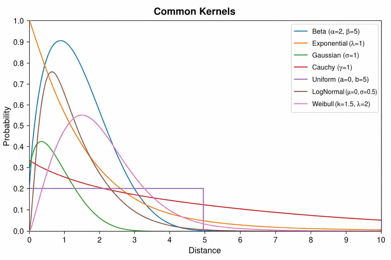
Each distance function is parameterised differently. Depending on the selected kernel, Biosecurity Commons will prompt for the appropriate parameter(s), such as a distance-decay coefficient, standard deviation, scale parameter or half-distance. These parameters determine the characteristic dispersal distance associated with the selected kernel, while the Distance Function determines the overall shape of the dispersal process. For information on other kernel distributions please checkout this guide.

 Best practice

Select a Distance Function that reflects the biology and dispersal mechanism of the target species. Where empirical information is unavailable, compare alternative kernels using sensitivity analyses to assess how assumptions about long-distance dispersal influence model predictions.

Gravity Parameters

Status:

• Required for Gravity Dispersal.

Available inputs:

The available parameters depend on the selected gravity formulation and typically include parameters controlling:

• destination attractiveness (node weights); and
• how movement declines with increasing distance.

Gravity Dispersal models movement between discrete source and destination locations (nodes). Unlike kernel-based dispersal, where destinations are sampled from a continuous distance distribution, Gravity Dispersal evaluates every potential destination and assigns each a relative probability of receiving dispersers.

Within Biosecurity Commons, the probability of movement is determined by two competing processes:

• Destination attractiveness, which increases the likelihood that dispersers move towards larger, more connected or otherwise more attractive destinations; and
• Distance decay, which reduces the likelihood of movement as the distance between the source and destination increases.

The relative probability of movement to each destination is proportional to its attractiveness and inversely related to the distance separating it from the source (Bossenbroek et al. 2001; Muirhead et al., 2006; Carrasco et al., 2010; Crespo-Pérez et al., 2011). These probabilities are then normalised so that they sum to one, allowing a destination to be sampled for each dispersal event.

This approach allows the model to represent situations where dispersers preferentially move towards important destinations while still accounting for the reduced likelihood of long-distance movements.

Example

Consider a network representing the movement of nursery stock between production properties. A large wholesale nursery may receive substantially more incoming consignments than a small retail outlet because it is both more attractive(greater connectivity or trade volume) and closer to many source locations. Gravity Dispersal captures this behaviour by preferentially directing movement towards highly attractive destinations while simultaneously reducing movement over longer travel distances

.

Best practice

Use Gravity Dispersal when movement occurs between known locations connected by transport, trade or movement pathways. Where possible, use destination weights that reflect the relative attractiveness or connectivity of each node, and select a distance-decay relationship consistent with the expected reduction in movement over distance.

Common mistake

Do not use Gravity Dispersal simply because movement occurs between spatial points. Gravity models are most appropriate when dispersal is influenced by both destination attractiveness and distance. If movement is independent of destination characteristics, a kernel-based or diffusion approach will generally provide a more appropriate representation.

Diffusion Rate

Status:

• Required for Diffusion and Reaction-Diffusion models.
• Raster grid models

Available inputs:

• Single value
• Spatial layer
• Temporal series
• Spatio-temporal dataset (where supported)

The Diffusion Rate controls the rate at which populations spread through space under diffusion-based dispersal models. Larger values produce more rapid spatial expansion, whereas smaller values restrict spread to locations closer to the invasion front.

Unlike kernel-based models, diffusion does not simulate independent long-distance movement events. Instead, populations expand continuously into neighbouring areas according to the specified diffusion rate.

Example

Increasing the Diffusion Rate causes the invasion front to expand more rapidly during each simulation time step, while reducing the rate produces slower, more gradual spread.

Best practice

Estimate diffusion rates from observed rates of range expansion where possible. Ensure the parameter is interpreted relative to the selected simulation time step.

Radial Spread Rate

Status:

• Required for Radial Diffusion.
• Spatially implicit model

Available inputs:

• Single value

The Radial Spread Rate specifies the distance by which the invasion boundary expands during each simulation time step. Unlike kernel or diffusion models, Radial Diffusion assumes populations spread uniformly outward from existing occupied areas.

This simple representation is computationally efficient and is most appropriate where spread can reasonably be approximated as a continuously expanding invasion front.

Example

A radial spread rate of 5 km per year causes occupied areas to expand outward by approximately five kilometres during each annual simulation time step.

Maximum Distance

Status:

• Required for most Kernel Dispersal functions in Raster models.
• Optional for Diffusion models in Raster models.
• Not applicable to Network models, Gravity Dispersal, or Radial Diffusion.

Available inputs:

• Single value (metres)

Maximum Distance specifies the greatest distance that a dispersal event may travel during a single simulation time step. This parameter is only available for Raster-based dispersal models.

For Kernel Dispersal, Maximum Distance defines the upper bound of the dispersal kernel. Distances are sampled from the selected probability distribution, but no dispersal event can exceed the specified maximum distance. Consequently, the Maximum Distance should represent the largest biologically plausible dispersal event expected within a single simulation time step.

For Diffusion models, Maximum Distance is optional and limits the maximum distance over which diffusion may occur during a single simulation time step. If left unspecified, no explicit upper limit is imposed.

In addition to its biological interpretation, Maximum Distance provides an important computational optimisation for raster models. Rather than evaluating every cell within the study region as a potential destination, Biosecurity Commons only evaluates cells located within the specified distance of each occupied source cell. This substantially reduces the number of dispersal calculations required during each simulation time step and can dramatically improve model performance for large study regions or high-resolution raster grids.

Because Network models operate on predefined nodes and connections rather than continuous raster cells, Maximum Distance is not required and is therefore not available.

Maximum Distance should always be interpreted relative to the selected simulation time step. For example, if annual time steps are used, it should represent the maximum distance an organism could realistically disperse in one year.

Example

Suppose annual simulation time steps are used to model the spread of an insect capable of dispersing up to 30 km in a single year.

Setting Maximum Distance = 30 km ensures that all simulated dispersal events remain within this biologically plausible limit. It also restricts dispersal calculations to raster cells located within 30 km of each occupied cell, substantially reducing computation time compared with evaluating the entire study region.

Best practice

Select a Maximum Distance that reflects the largest biologically plausible dispersal event over a single simulation time step. Avoid unnecessarily large values, particularly for raster models, as these increase the number of raster cells evaluated during each dispersal event and may substantially increase computation time. Where empirical data are unavailable, use published observations or expert elicitation and evaluate alternative values through sensitivity analyses.

Common mistake

Do not confuse Maximum Distance with the typical dispersal distance. Most dispersal events will occur over much shorter distances, with the characteristic dispersal behaviour determined by the selected dispersal function and its associated parameters. Maximum Distance simply defines the upper limit of the dispersal process. Likewise, avoid specifying excessively large values "just to be safe", as this can substantially increase computation time without improving biological realism.

Modify Dispersal

The parameters in this section modify the underlying dispersal process to better represent biological or environmental processes that influence movement. Unlike the parameters described previously, these settings do not determine how dispersers are generated or the fundamental mechanism of movement. Instead, they refine how the selected dispersal function is realised during the simulation.

These modifiers are optional and should generally be used only where there is biological or empirical evidence that they improve the realism of the model. Examples include prevailing winds or ocean currents that bias movement direction, habitat features that attract dispersers, or landscape characteristics that facilitate or impede movement.

Because these parameters modify rather than replace the underlying dispersal process, users should first ensure that the selected dispersal function has been appropriately parameterised before introducing additional modifiers.

Direction Function

Status:

• Optional.

Available inputs:

• Uniform (default)
• Beta distribution
• User-defined lookup table (CSV)

The Direction Function modifies the underlying dispersal process by biasing the direction in which dispersers move. By default, dispersal is assumed to be isotropic, meaning dispersers are equally likely to move in any direction. Where directional movement is expected, users may specify a directional probability distribution that preferentially directs dispersal towards particular bearings.

Biosecurity Commons supports three directional functions:

• Uniform, where all directions are equally likely (default when direction not-specified).
• Beta distribution, parameterised using Alpha, Beta and an optional Shift parameter to control both the strength and orientation of directional bias.
• User-defined lookup table, allowing users to specify the relative probability associated with each direction (in degrees) using a CSV file.

The selected directional function is applied uniformly across the entire study region. Consequently, all dispersal events are sampled from the same directional probability distribution, regardless of their geographic location. This approach is intended to represent broad-scale directional drivers, such as prevailing winds, dominant ocean currents, or regional topographic gradients, but does not account for local spatial variation in movement direction. Users can also specify whether directional probabilities describe movement towards a specified direction (e.g. bird migration) or from a specified direction (e.g. wind-driven dispersal). The default is towards.

Example

A fungal pathogen dispersed predominantly by prevailing westerly winds could be modelled using a directional distribution centered on the prevailing wind direction. Every dispersal event throughout the study region would exhibit the same directional bias, increasing the probability of eastward spread.

Best practice

Use the Direction Function only where there is biological or empirical evidence that dispersal exhibits a consistent directional bias across the study region. Where possible, parameterise the directional distribution using observed movement data or expert knowledge.

Attractors

Status

• Optional.

Available inputs

Raster models

• Raster layer(s)

Network models

• CSV containing node weights

Attractors modify the probability that dispersers move towards particular destinations. Rather than influencing how far dispersers travel, attractors influence where dispersers are most likely to arrive once a dispersal event has been generated.

Attractors represent the relative attractiveness of potential destination locations and may be derived from a wide range of biological or operational factors, including habitat suitability, host abundance, resource availability, transport infrastructure, human population density or other landscape features that influence destination selection.

For many species, attractors represent behavioural preferences, where dispersing individuals actively select destinations offering favourable resources or environmental conditions. For example, vertebrates may preferentially move towards suitable habitat, food resources or breeding sites, while insects may preferentially colonise areas containing abundant host plants. In other applications, attractors may represent human-assisted movement pathways, such as freight terminals, ports or transport hubs that increase the likelihood of long-distance movement.

For raster models, attractors are provided as one or more raster layers. For network models, they are supplied as node-specific relative weights. Where multiple attractors are provided, Biosecurity Commons multiplies the individual layers together to derive an overall destination attractiveness surface or node weighting. Locations with larger combined values therefore have a greater probability of receiving dispersers.

Example

Suitable habitat may be used as an attractor when modelling the movement of vertebrates that actively select preferred habitat during dispersal. Likewise, host density may be used to increase the probability that insect pests colonise areas containing abundant host plants. For human-assisted spread, transport hubs or freight terminals may be represented as highly attractive destinations because they receive relatively large volumes of incoming material.

Additional examples of attractor variables can be found in Schneider et al (1998), Bossenbroek et al. (2001); Muirhead et al., (2006); Carrasco et al., (2010); Crespo-Pérez et al., (2011).

Best practice

Use attractors to represent processes that influence destination selection rather than establishment. Where multiple independent factors influence movement behaviour, provide separate attractor layers rather than combining them manually, allowing Biosecurity Commons to calculate their combined effect consistently.

Permeability

Status:

• Optional.

Available inputs

Raster models

• Raster layer containing permeability values between 0 and 1.

Network models

• Table containing connected node pairs and the permeability of each path.

Permeability represents the relative ease with which dispersers move through raster cells or along paths between network nodes. Unlike Attractors, which influence the relative probability of selecting a destination, permeability modifies the effective distance required to move through the landscape or network.

Permeability values range between 0 and 1, where:

• 1 indicates unrestricted movement and does not alter the effective distance;
• 0 prevents movement through the cell or along the network path; and
• intermediate values increase the effective distance required to traverse that cell or path.

Biosecurity Commons applies the inverse of permeability to scale physical distance (Etherington 2016). For example, a permeability of 0.5makes the effective distance twice the actual distance, while a permeability of 0.2 makes it five times the actual distance. Dispersers therefore exhaust their available dispersal distance more quickly when moving through low-permeability environments.

Permeability can represent natural or artificial features that facilitate or impede movement, including vegetation types, land cover, topography, rivers, roads, urban areas, fences or differences in transport connectivity. Values may be derived from empirical movement studies, resistance or least-cost analyses, expert elicitation, or by assigning relative permeability values to mapped landscape classes.

Example

Suppose an invasive mammal has an available dispersal distance of 1000 m during one simulation time step and encounters a fence represented by a 100 m-wide raster cell.

• With permeability 1.0, crossing the cell uses 100 m of its dispersal distance.
• With permeability 0.5, the same cell has an effective distance of 200 m.
• With permeability 0.2, it has an effective distance of 500 m.
• With permeability 0, the fence acts as a complete barrier and cannot be crossed.

A partially effective fence can therefore be represented using an intermediate permeability value, while an impermeable exclusion fence may be represented using zero. In a network model, the same principle is used to make particular connections easier or more difficult to traverse.

Best practice

Use permeability to represent relative resistance to movement. Where possible, derive values from empirical movement data, published resistance estimates or structured expert elicitation. Because permeability is applied inversely, small values can produce very large increases in effective distance; sensitivity analysis is therefore particularly important.

Common mistake

Do not interpret permeability values as the probability that an organism successfully crosses a landscape feature. Instead, permeability modifies the effective distance travelled through the landscape. Lower permeability values make movement progressively more difficult, but the resulting reduction in dispersal depends on the selected dispersal function.

Simulating Impacts (Optional)

Population spread models estimate where invasive species establish, how populations grow and how they spread. However, for most biosecurity applications, understanding the consequences of invasion is just as important as predicting its spread. Management decisions are typically driven by the impacts an invasive species is expected to cause, including economic losses, environmental degradation, reduced ecosystem services and social or cultural consequences (Dodd et al. 2020).

Impact models extend population spread simulations by translating the predicted distribution and abundance of an invasive species into estimates of these consequences. This enables users to quantify how impacts develop through time, identify the assets most at risk, compare alternative management strategies, and evaluate the benefits of surveillance, containment and eradication programs.

Within Biosecurity Commons, impacts are calculated dynamically throughout the simulation using the predicted distribution and abundance of the invasive species. Depending on the selected Impact Model, impacts may accumulate through time, recover following successful management, or dynamically influence subsequent invasion processes through feedbacks to Threat Suitability, Carrying Capacity or Dispersal Attractors. This enables users to represent not only the consequences of invasion, but also ecological systems in which changing resource availability influences future spread.

The way impacts are specified depends on the selected Spatial Framework. For Raster models, assets are represented using raster datasets describing their spatial distribution and value. For Network models, assets are associated with individual nodes, such as farms, ports or other facilities. For Spatially Implicit models, assets are specified for the implicit area of interest. Consequently, impact datasets should always be prepared using the same spatial framework as the spread model.

Multiple impacts may be simulated simultaneously. For example, a single simulation may independently estimate agricultural production losses, biodiversity impacts, infrastructure damage and ecosystem service degradation, providing a more comprehensive assessment of the consequences of invasion.

Which Impact Model Should I Choose?

 Monetary Impact

The Monetary Impact model estimates the economic consequences of an invasive species by applying impacts to assets expressed in monetary terms (Dodd et al. 2020; Stoeckl et al. 2023). Assets may include agricultural production, forestry, livestock, infrastructure, environmental assets or any other resource for which an economic value can be assigned.

Monetary impacts accumulate throughout the simulation according to the duration and severity of infestation. Optional recovery and depreciation parameters allow users to account for delayed recovery following management and changes in asset value through time, such as discounting or inflation.

This model is most appropriate where the primary objective is to quantify economic losses or compare the costs and benefits of alternative management strategies.

Recommended applications

• Agricultural production losses.
• Forestry production.
• Livestock industries.
• Infrastructure damage.
• Cost-benefit analyses.
• Economic evaluation of surveillance and management programs.

Advantages

• Produces impacts in readily interpretable monetary units.
• Supports economic evaluation of management strategies.
• Allows recovery following successful management.
• Supports depreciation and discounting of future asset values.

Limitations

• Requires reliable monetary valuation of affected assets.
• May not adequately capture environmental or social values that are difficult to monetise.
• Does not explicitly represent ecological feedbacks unless Dynamic Impact modelling is used.

Non-monetary Impact

The Non-monetary Impact model estimates impacts using user-defined quantitative measures rather than monetary values. This allows users to represent environmental, ecological or social impacts that are difficult or inappropriate to express economically.

Assets may represent habitat area, habitat condition (e.g. HCAS; Valavi et al. 2025) biodiversity value, ecosystem services, cultural assets, recreational value or any other measurable indicator of interest. Recovery parameters allow assets to return towards their original condition following successful management.

This model is most appropriate where the objective is to quantify changes in environmental or social assets rather than economic losses.

Recommended applications

• Biodiversity impacts.
• Habitat degradation.
• Ecosystem services.
• Cultural heritage.
• Social impacts.
• Conservation planning.

Advantages

• Suitable for environmental and social assessments.
• Supports any user-defined impact metric.
• Allows recovery following successful management.
• Straightforward to interpret using meaningful ecological indicators.

Limitations

• Does not directly estimate economic losses.
• Requires users to define appropriate impact metrics.
• Does not represent dynamic feedbacks unless Dynamic Impact modelling is used.

Dynamic Impact

The Dynamic Impact model represents assets that change through time as a consequence of invasion. Rather than simply recording impacts, the remaining condition or quantity of the asset is updated continuously throughout the simulation.

A key feature of the Dynamic Impact model is its ability to create feedbacks between impacts and invasion dynamics. As assets are depleted or recover, they may be used to modify Threat Suitability, Carrying Capacity or Dispersal Attractors, allowing changes in resource availability to influence future establishment, population growth or dispersal.

This approach is particularly useful where the invasive species alters the very resources that determine its subsequent spread or persistence.

Recommended applications

• Host depletion.
• Plantation biomass.
• Food resources.
• Habitat degradation.
• Resource availability.
• Ecological feedbacks.

Advantages

• Represents changing asset condition through time.
• Supports recovery following management.
• Allows impacts to modify subsequent invasion dynamics.
• Provides the most biologically realistic representation where resources influence future spread.

Limitations

• Requires greater biological understanding of feedback processes.
• More complex to parameterise than the other impact models.
• Appropriate only where impacts genuinely alter future invasion dynamics.

Configure Impact Parameters

Once an Impact Model has been selected, users specify the assets being affected and how those assets respond to invasion. Most parameters are shared across all Impact Models, allowing the same assets and impact relationships to be represented using either Monetary, Non-monetary or Dynamic impacts. Additional parameters are only required where the selected Impact Model supports capabilities such as depreciation or dynamic feedbacks.

As with previous workflow stages, the format of each input depends on the selected Spatial Framework. Raster models require raster datasets describing the spatial distribution of assets, Network models associate asset values with individual nodes, and Spatially Implicit models define asset values for each management unit or region. All impact datasets should therefore be prepared using the same Spatial Framework as the spread model.

The following sections describe the parameters common to all Impact Models, followed by those specific to the Monetary and Dynamic Impact models.

Asset Name

Status:

• Required.

The Asset Name provides a descriptive label for the impacted asset. This name is used throughout the simulation outputs and visualisations to distinguish between multiple impact layers.

Best practice

Use descriptive names that clearly identify the asset being modelled.

Asset Data

Status:

• Required.

Available inputs:

Raster models

• Raster layer.

Network models

• CSV containing asset values for each node.

Spatially Implicit models

• Table containing asset values for each management unit or region.

Asset Data define the location and magnitude of the assets that may be impacted by the invasive species. Assets may represent monetary value, crop production, livestock numbers, timber volume, habitat area, biodiversity value, ecosystem services, infrastructure, human populations, or any other quantity relevant to the modelling objective. Biosecurity Commons includes a range of curated monetary and non-monetary (e.g. HCAS) asset datasets that can be used directly within impact models, although users may also upload their own custom asset data where appropriate.

The format of the Asset Data depends on the selected Spatial Framework. For Raster models, each raster cell contains the asset value at that location. For Network models, values are associated with individual nodes such as farms or ports. For Spatially Implicit models, values are specified for each management unit or region.

Multiple asset datasets may be defined within a single simulation, allowing different assets to be impacted independently. For example, a single simulation may simultaneously estimate impacts to agricultural production, biodiversity, infrastructure and ecosystem services.

Example

A forestry model may use a raster describing the annual value of standing timber across the landscape, while a livestock disease model may associate the annual production value of livestock with individual farm nodes. A regional planning model may specify the total annual agricultural production value for each administrative region.

Best practice

Ensure the Asset Data use the same Spatial Framework and spatial extent as the spread model and represent the asset values at the temporal resolution specified by the Temporal Units parameter.

Asset Units

Status:

• Required.

Asset Units define the quantity represented by the Asset Data. Examples include AUD, tonnes, hectares, livestock head, biomass, habitat quality score, or any other quantitative measure relevant to the analysis.

Temporal Units

Status:

• Required.
• Monetary Impact models only.

Available inputs

• Per time step
• Per annum

Temporal Units specify the time period represented by the monetary Asset Data. For example, agricultural production may be provided as an per annum or per time step.

Biosecurity Commons automatically converts these values to the simulation time step. Consequently, users can provide asset values using either per annum without needing to manually adjust them to match the simulation.

For example, if annual production values are supplied but the simulation uses monthly time steps, the platform converts the annual values into equivalent monthly values before calculating impacts. Likewise, if a simulation uses weekly time steps, the annual values are converted to weekly values.

Best practice

Specify the temporal units that correspond to the original Asset Data rather than manually converting values to the simulation time step.

Loss Fraction

Status:

• Required.

Available inputs:

• Single value between 0 and 1.

The Loss Fraction defines the proportion of the affected asset lost when the invasive species causes an impact. Values range between 0 and 1, where:

• 0 represents no loss;
• 0.2 represents a 20% loss; and
• 1 represents complete loss of the affected asset.

The Loss Fraction is specified as a constant and does not vary across space or through time. Instead, spatial and temporal variation in realised impacts arises from:

• the distribution and value of the asset;
• whether the invasive species is present at a location; and
• for density-based impacts, the simulated abundance of the threat relative to carrying capacity.

Consequently, two locations may experience different realised impacts even when the same Loss Fraction is applied, because they may contain different asset values or support different threat abundances.

Example

Suppose the Loss Fraction is 0.2.

If a location contains an asset valued at AUD 100,000 and the threat causes the full specified impact, the loss is AUD 20,000.

If another location contains an asset valued at AUD 40,000, the same Loss Fraction produces a loss of AUD 8,000.

For a density-based impact, the realised loss may be lower where the threat population is below carrying capacity because the Loss Fraction is scaled by relative population density.

Best practice

Base the Loss Fraction on published impact studies, experimental data or structured expert elicitation. Interpret it as the maximum proportional loss associated with the selected impact relationship.

Impact Type

Status:

• Optional - defaults to Presence-based.

Applies to:

• Unstructured Population Model.
• Stage-structured Population Model.

Impact Type determines how impacts are related to the simulated population.

Two options are available:

• Presence-based, where impacts occur whenever the invasive species is present.
• Density-based, where impacts scale according to simulated population abundance relative to the carrying capacity.

Presence-based impacts are appropriate where even small populations produce substantial impacts. Density-based impacts are better suited to situations where impacts increase progressively as populations become larger.

Example

An exotic pathogen may trigger quarantine restrictions immediately following detection, making a Presence-based impact appropriate. In contrast, crop damage caused by an insect pest may increase as population density increases, making a Density-based impact more appropriate.

Best practice

Choose the Impact Type that best reflects the biological relationship between population abundance and asset damage.

Impact Stages

Status:

• Optional.

Applies to:

• Stage-structured Population Model.

Impact Stages specify which life stages contribute to impacts. Different life stages often differ substantially in the damage they cause. For example, larval stages may consume host material, whereas adults are responsible primarily for dispersal and reproduction.

Selecting only the relevant life stages allows impacts to better reflect the biology of the species.

Example

For many defoliating insects, only larval stages contribute to vegetation loss, whereas adult stages produce little direct damage.

Best practice

Include only those life stages known to contribute meaningfully to the impacted asset.

Asset Recovery Delay

Status:

• Optional.

Available inputs:

• Single value expressed in simulation time steps.

Asset Recovery Delay specifies the time required for an impacted asset to recover to its original value or condition following successful removal of the invasive species.

Recovery occurs progressively over the specified period rather than instantaneously. Smaller values represent assets that recover rapidly, whereas larger values represent assets requiring longer to return to their pre-impact condition.

The value should be interpreted relative to the selected simulation time step. For example, if the simulation uses annual time steps and an asset requires 20 years to fully recover, the Asset Recovery Delay should be specified as 20.

Example

Consider a pine plantation affected by an invasive wood-boring beetle. Following successful eradication of the pest, the plantation must be replanted and allowed to regrow before timber production returns to its original value.

If the plantation is expected to take 25 years to reach its pre-infestation value, the Asset Recovery Delay should be specified as:

• 25 for annual simulation time steps; or
• 300 for monthly simulation time steps.

Biosecurity Commons then progressively restores the asset value over this period until it reaches its original level.

Best practice

Estimate the recovery period using published information, historical observations or expert knowledge, and ensure the value is expressed using the same temporal resolution as the simulation.

Depreciation

Status

• Optional.
• Monetary Impacts

Depreciation allows the value of an asset to change through time independently of the invasive species. This is typically used to represent discounting, inflation or other economic processes affecting future asset values.

Depreciation is applied independently of invasion impacts and therefore represents changes in asset value that would have occurred even if the invasion had not taken place.

Example

Future agricultural losses may be discounted to present-day values when evaluating long-term management strategies.

Best practice

It is common practice to apply real discount rates between 3% and 7% in agricultural economic analyses. For environmental assets and ecosystem services, lower discount rates are often recommended to better reflect their long-term value and the fact that their benefits may persist indefinitely (i.e. Depreciation of 0) rather than depreciating over time.

Dynamic Feedback

Status:

• Optional.
• Dynamic impacts

Available options:

• Threat Suitability.
• Carrying Capacity.
• Attractors.

Dynamic Feedback allows changes in the impacted asset to modify subsequent invasion dynamics.

Depending on the selected option, reductions in asset condition may modify:

• Threat Suitability, altering the probability of successful establishment.
• Carrying Capacity, changing the maximum population supported at each location.
• Attractors, modifying the relative attractiveness of locations for future dispersal.

This enables users to represent ecological feedbacks where the invasive species progressively alters the environment, and those changes subsequently influence future spread.

Example

Progressive depletion of host plants may reduce Threat Suitability, declining food resources may reduce Carrying Capacity, and degradation of habitat may reduce Attractors, making locations less attractive to future dispersers.

Best practice

Only enable Dynamic Feedback where there is biological evidence that changes in the impacted asset influence future establishment, population growth or dispersal.

Simulating Actions (Optional)

Population spread models estimate how invasive species establish, grow and spread. However, one of the primary objectives of biosecurity modelling is to evaluate how management interventions alter the trajectory of an invasion. Action models extend population spread simulations by allowing users to simulate surveillance, control and removal activities, enabling alternative management strategies to be compared under realistic invasion scenarios.

Within Biosecurity Commons, actions are applied dynamically throughout the simulation and interact directly with the simulated population. Depending on the selected Action Model, actions may detect previously undetected populations, suppress population growth or spread, reduce the probability of establishment, or remove populations entirely. This enables users to evaluate the effectiveness, costs and long-term consequences of different management strategies.

The way actions are specified depends on the selected Spatial Framework. Raster models typically use raster datasets describing where management actions occur or how effective they are. Network models associate actions with individual nodes, such as farms, ports or surveillance sites. Spatially Implicit models specify actions the implicit area of interest.

Multiple actions may be defined within a single simulation. Actions are executed sequentially in the order they are specified, allowing users to construct complex management programs consisting of multiple complementary interventions. For example, a simulation may first apply surveillance to detect infestations, followed by search and destroy of detected populations, growth suppression through chemical control, and finally spread control to reduce further dispersal. The order of actions can influence simulation outcomes and should therefore reflect the intended management program.

Which Action Model Should I Choose?

Detection (Surveillance)

The Detection (Surveillance) Action Model represents surveillance activities undertaken to detect invasive species. Unlike Control or Removal actions, surveillance does not directly alter population growth or spread. Instead, it determines whether infestations are successfully detected based on the surveillance sensitivity specified for each location.

Surveillance may represent a wide range of biosecurity activities, including field inspections, trapping programs, environmental sampling, diagnostic testing, community surveillance, or other monitoring systems. Detection is modelled probabilistically, allowing infestations to remain undetected despite surveillance when detection sensitivity is imperfect.

The probability of detecting an infestation is determined by a location-specific surveillance sensitivity layer. This layer may be uploaded directly by the user or generated using the Surveillance Design workflow within Biosecurity Commons. The Surveillance Design workflow combines information on surveillance effort, sampling strategy and detection efficacy to estimate the probability of detecting an infestation at each location. These spatially explicit detection probabilities can then be used directly within Action models, ensuring surveillance simulations are based on realistic surveillance system performance rather than arbitrary assumptions.

Detection actions are particularly useful for evaluating early detection programs, estimating expected time to detection and comparing alternative surveillance strategies.

Recommended applications

• Early detection surveillance.
• Delimitation surveys.
• General surveillance.
• Monitoring established infestations.
• Evaluating surveillance strategies.
• Estimating expected time to detection.
• Supporting Search & Destroy programs.

How detection works

At each simulation time step, the model evaluates every occupied location included within the surveillance program.

For each location, the probability of successfully detecting the population is determined by the surveillance sensitivity supplied by the user. If detection occurs, the location is recorded as detected for that simulation step. Unless another management action is configured (for example Search & Destroy or Removal), the population continues to grow and disperse normally after detection.

Because detection is modelled probabilistically, identical surveillance programs will generally produce different detection outcomes between simulation replicates. Running multiple replicates therefore allows users to estimate quantities such as the expected number of detections, variability in surveillance performance, and expected detection timing.

Surveillance Sensitivity

Status:

• Required.

Available inputs:

Raster models

• Raster layer (GeoTIFF).

Network models

• CSV containing lon, lat and sensitivity columns.

Spatially Implicit models

• Single value.

Surveillance Sensitivity defines the probability that surveillance successfully detects the selected Detection Target during each scheduled surveillance event. 

Surveillance sensitivity represents the combined effectiveness of the surveillance system, incorporating factors such as sampling intensity, diagnostic accuracy, inspector performance, pest detectability and environmental conditions. The supplied value or spatial layer is applied consistently each time surveillance is undertaken. Changes in surveillance effort through time are represented using the Schedule parameter rather than by varying surveillance sensitivity.

Surveillance sensitivity may be specified directly by the user or generated using the Surveillance Design workflow within Biosecurity Commons. The Surveillance Design workflow estimates location-specific detection probabilities that can be imported directly into Population Spread Modelling, allowing surveillance actions to be based on a quantitatively designed surveillance system rather than assumed values.

Example

A trapping network may have a surveillance sensitivity ranging from 0.15 in sparsely monitored regions to 0.80 around high-priority surveillance sites, reflecting differences in surveillance effort and expected detection performance.

Detection Target

Status:

• Required for Unstructured and Stage-structured population models.

Available options:

• Presence
• Population Size (Threshold)
• Individual Organisms

The Detection Target defines how the supplied Surveillance Sensitivity is interpreted when calculating the probability of detection. Selecting the appropriate option ensures that the surveillance model is consistent with both the underlying population model and the way surveillance sensitivity has been estimated.

The available options are interpreted as follows:

• Presence – Surveillance Sensitivity represents the probability of detecting any occupied location, regardless of the number of detectable individuals present. Detection probability is therefore independent of population size. This option is equivalent to using a Population Threshold of one detectable individual and is typically appropriate when surveillance sensitivity has been estimated as the probability of detecting an infestation or occupied site.
• Population Size (Threshold) – Surveillance Sensitivity represents the probability of detecting a local population containing at least a specified number of detectable individuals (the Population Threshold). For populations larger than or equal to the threshold, the supplied surveillance sensitivity is applied directly. For populations smaller than the threshold, Biosecurity Commons reduces the detection probability proportionally according to the ratio of the simulated population size to the threshold value. This option is useful when surveillance performance has been estimated for populations of a known minimum size rather than individual organisms.
• Individual Organisms (default) – Surveillance Sensitivity represents the probability of detecting each detectable individual independently. Biosecurity Commons combines these individual detection probabilities to calculate the overall probability of detecting the local population. Consequently, larger populations become progressively more likely to be detected than smaller populations.

Selecting the appropriate Detection Target is important because the same surveillance sensitivity may produce very different detection probabilities depending on how it is interpreted.

Population Threshold

Status:

• Required when Population Size (Threshold) is selected.

The Population Threshold specifies the minimum number of detectable individuals for which the supplied surveillance sensitivity applies.

When the simulated population is greater than or equal to the threshold, the specified surveillance sensitivity is used directly. When the simulated population is smaller than the threshold, the probability of detection is reduced proportionally according to:

Detection Probability = Surveillance Sensitivity × (Population Size ÷ Population Threshold)

This allows surveillance performance to increase naturally as populations grow towards the size for which surveillance sensitivity was originally estimated.

Example

Suppose surveillance has an 80% probability of detecting populations containing at least 100 detectable individuals.

• A population of 100 individuals has a detection probability of 0.80.
• A population of 50 individuals has a detection probability of 0.40.
• A population of 25 individuals has a detection probability of 0.20. 

Detectable Stages

Status:

• Optional (Stage-structured population models only).

For Stage-structured population models, users may specify which life stages are detectable by the surveillance system.

This allows surveillance systems to reflect biological reality where only particular life stages can be reliably detected. For example, surveillance may target adults using traps, eggs during visual inspections, or symptomatic host material.

Only the selected life stages contribute to the probability of detection during surveillance.

Example

A pheromone trapping program for an insect pest may detect only adults, whereas visual inspections may detect larvae and adults.

Control

The Control Action Model represents management interventions that reduce the ability of an invasive species to establish, grow or spread. Unlike the Removal Action Model, which eliminates populations from treated locations, control actions modify one or more biological processes governing invasion dynamics, allowing surviving populations to persist.

Rather than representing control as a single process, Biosecurity Commons provides four complementary control mechanisms that target different stages of the invasion process. These mechanisms may be used individually or combined within the same simulation to represent integrated management programs.

Each control mechanism acts on a different component of the invasion process and may therefore be combined to represent realistic management programs. For example, an eradication program may first use Search & Destroy to locate and remove known infestations, Growth Control to suppress any undetected populations that remain, and Spread Control to reduce the likelihood of further dispersal beyond the containment area. Likewise, Establishment Control may be applied proactively around high-risk locations to reduce the probability that new introductions establish.

Search & Destroy

Search & Destroy represents management programs that combine surveillance and removal into a single management action. Rather than configuring separate Detection and Removal actions, Search & Destroy models the complete management process by accounting for both the probability of detecting an infestation and the probability of successfully removing it once detected.

This approach is well suited to eradication programs where surveillance and treatment occur as part of the same operational response, such as delimitation surveys (Hauser et al. 2016) followed immediately by destruction of infested hosts, targeted pesticide applications, or removal of infected plants (Hauser & McCarthy 2009).

Because removal can only occur after an infestation has been detected, the overall probability of successful management depends on both the effectiveness of the surveillance system and the effectiveness of the removal method. Consequently, Search & Destroy provides a convenient and biologically realistic way of representing integrated surveillance and response programs.

Typical applications include:

• Eradication programs.
• Delimitation surveys followed by treatment.
• Search and treatment campaigns.
• Rapid response to new incursions.
• Ongoing surveillance and removal programs.

Applicability

How Search & Destroy Works

At each scheduled management event, Biosecurity Commons evaluates every occupied location included within the management program.

Search & Destroy combines two probabilistic processes:

1. successful detection of an infestation; and
2. successful removal of the detected infestation.

Rather than specifying these processes independently, Search & Destroy represents their joint probability of successusing a single Control Effectiveness parameter. Consequently, successful management can only occur when an infestation is both detected and successfully removed during the same management event.

Where independent estimates of detection and removal success are available, the joint probability may be approximated as:

Management Success = Detection Success × Removal Success

For example, if surveillance detects infestations with a probability of 0.80 and removal succeeds with a probability of 0.90, the corresponding Control Effectiveness is:

0.80 × 0.90 = 0.72

Conceptually, this implementation is equivalent to applying a Detection action immediately followed by a Removal action within the same simulation time step, but provides a simpler and more efficient representation of integrated search and treatment programs.

Search & Destroy uses the following unique parameters:

• Control Effectiveness Type (Unstructured and Stage-structured Population Models only).
• Controlled Stages (Stage-structured Population Models only).

The remaining parameters are described in the Shared Control Parameters section.

Growth Control

Growth Control represents management interventions that suppress the growth of established populations. Rather than attempting to detect or remove infestations, Growth Control reduces the rate at which local populations increase through time. Consequently, treated populations continue to persist but grow more slowly, reducing future spread, delaying invasion progression and lowering overall abundance.

Growth Control is particularly well suited to representing interventions that reduce reproduction or survival, including chemical control, biological control, sterile insect techniques, grazing, culling, or other management activities that suppress populations without necessarily eliminating them.

Typical applications include:

• Chemical control.
• Biological control.
• Sterile insect releases.
• Grazing or browsing.
• Population suppression programs.
• Long-term integrated pest management.

Applicability

How Growth Control Works

At each scheduled management event, Biosecurity Commons modifies the demographic processes responsible for population growth.

Unlike Search & Destroy, Growth Control does not remove existing infestations. Instead, it suppresses population growth by reducing reproduction, increasing mortality, or both, depending on the selected configuration.

Repeated management therefore produces smaller local populations through time, reducing both the abundance of the invasive species and the number of individuals available for future dispersal.

Growth Control is particularly useful where eradication is unlikely but sustained population suppression can substantially reduce long-term impacts.

Growth Control includes the following unique parameters:

• Apply To (Stage-structured Population Models only).
• Controlled Stages (Stage-structured Population Models only).

The remaining parameters are described in the Shared Control Parameters section.

Spread Control

Spread Control represents management interventions that reduce the successful movement of invasive species between locations. Rather than suppressing local populations, Spread Control acts directly on the dispersal process, reducing the probability that individuals successfully move to new locations.

Spread Control is particularly well suited to representing interventions that limit movement pathways, including quarantine, movement restrictions, vehicle decontamination, exclusion fencing, transport inspections, and containment zones.

Typical applications include:

• Quarantine.
• Movement restrictions.
• Vehicle wash-down stations.
• Transport inspections.
• Exclusion fencing.
• Containment zones.

Applicability

How Spread Control Works

At each scheduled management event, Biosecurity Commons reduces the probability that dispersal events successfully occur from managed locations.

Unlike Growth Control, existing populations continue to grow normally. Instead, Spread Control reduces the likelihood that dispersers successfully reach new locations, slowing the spatial expansion of the invasion without directly affecting local population abundance.

Spread Control is therefore most appropriate for evaluating containment strategies that aim to restrict movement rather than suppress existing infestations.

Spread Control has no unique configuration parameters. All configuration is performed using the Shared Control Parameters described below.

Establishment Control

Establishment Control represents management interventions that reduce the probability that newly arriving individuals successfully establish following dispersal. Unlike Spread Control, which reduces movement between locations, Establishment Control assumes dispersal has already occurred and instead reduces establishment success at the destination.

Establishment Control is particularly well suited to representing preventative management strategies such as resistant host varieties, vaccination, habitat modification, prophylactic pesticide applications, environmental sanitation, or other measures that reduce the likelihood of establishment without affecting dispersal.

Typical applications include:

• Resistant host varieties.
• Habitat modification.
• Vaccination.
• Prophylactic treatments.
• Environmental sanitation.
• Preventative biosecurity programs.

Applicability

How Establishment Control Works

At each scheduled management event, Biosecurity Commons reduces the probability that dispersers successfully establish after arriving at managed locations.

Existing populations are unaffected. Instead, Establishment Control acts only on new establishment events occurring while management is active. Consequently, it is particularly useful for evaluating preventative management strategies designed to reduce invasion risk before populations become established.

By reducing establishment success rather than growth or spread, Establishment Control can substantially delay invasion progression while allowing existing infestations to persist.

Removal

The Removal Action Model represents the direct removal of invasive species from the simulated population. Unlike Search & Destroy, which assumes removal occurs immediately following successful detection and represents the two processes using a single joint probability, Removal separates the removal process from surveillance. This allows users to model detection and removal as independent actions, each with their own probabilities, schedules, costs and spatial configurations.

Removal can represent a wide range of biosecurity interventions, including trapping, culling, hand removal, destruction of infested plants or animals, pesticide applications, harvesting, sanitation activities, or other management actions that directly reduce population abundance. Depending on the selected population model, removal may act on entire local populations or individual organisms, and Stage-structured Population Models can further restrict removal to selected life stages.

Removal actions are particularly useful when surveillance and management need to be modelled independently, allowing users to evaluate how different surveillance systems influence management outcomes or to represent management programs that occur independently of formal surveillance.

Recommended applications

• Routine trapping or culling programs.
• Herbicide or pesticide applications.
• Destruction of infested plants, animals or materials.
• Public reporting and removal programs.
• Ongoing suppression programs.
• Evaluating surveillance-dependent versus surveillance-independent management.
• Building custom surveillance and response workflows using separate Detection and Removal actions.

Applicability

How Removal Works

At each scheduled management event, Biosecurity Commons evaluates whether removal is applied to occupied locations.

By default, removal is linked to surveillance. When one or more Detection actions are included within the simulation, removal is only attempted at locations that have been successfully detected during the current simulation time step.

Alternatively, users may enable Always Apply Removal, allowing removal to occur whenever the invasive species is present, regardless of whether it has been detected. This option is useful for representing routine management, incidental removal by the public, or ongoing suppression programs that operate independently of formal surveillance.

Once removal is triggered, Biosecurity Commons applies the specified Removal Probability to determine whether removal is successful. Depending on the selected Removal Probability Type, this probability may apply to either the entire local population or to individual organisms.

Removal actions may therefore be used independently or combined with Detection actions to represent a wide range of management strategies, from passive public removal through to highly structured surveillance-response programs.

Removal Probability Type

Status:

• Required for Unstructured and Stage-structured Population Models.
• Not applicable to Presence-only Population Models.

The Removal Probability Type defines how the supplied Removal Probability is interpreted.

Example

Suppose the Removal Probability is 0.8.

• Population: each occupied location has an 80% probability of complete removal.
• Individual: each removable individual has an 80% probability of removal, allowing partial population suppression where some individuals survive.

Best practice

Select the interpretation that matches how removal effectiveness has been estimated.

Always Apply Removal

Status:

• Optional.

Always Apply Removal determines whether removal is dependent on surveillance.

When disabled (default), removal is only attempted at locations that have been successfully detected by one or more Detection actions during the simulation.

When enabled, removal is applied whenever the invasive species is present, regardless of whether detection has occurred. This allows users to represent background removal processes such as routine control programs, public removal of weeds, or ongoing management undertaken independently of formal surveillance.

Example

A local council may routinely remove invasive weeds whenever they are encountered during maintenance activities, regardless of whether they were detected through a formal surveillance program. Enabling Always Apply Removal represents this ongoing background management.

Best practice

Enable this option only where removal genuinely occurs independently of surveillance.

Common mistake

Do not enable Always Apply Removal when modelling reactive eradication programs. In these situations, removal should normally depend on successful detection.

Only Remove Detected Individuals

Status:

• Optional.
• Available only when Individual Removal Probability is selected and Detection actions are included.

When Individual removal is selected, this option specifies whether removal is applied only to the individuals that have been detected.

When enabled, only detected individuals are eligible for removal, representing management methods such as trapping where only captured individuals are removed.

When disabled, removal is applied to all individuals present at locations where the infestation has been detected. This represents management activities such as pesticide application or treatment of an entire property following detection.

Example

A trapping program removes only insects captured in traps and therefore would typically enable Only Remove Detected Individuals. By contrast, a herbicide application treats the entire infestation following detection and would typically leave this option disabled.

Removable Stages

Status

• Required for Stage-structured Population Models only.

Removable Stages specifies which life stages are susceptible to removal.

Only the selected stages are considered when applying the Removal action, allowing management to target biologically realistic portions of the life cycle.

Example

A pheromone trapping program may remove only adult insects, whereas destruction of infested nursery stock may remove eggs and larvae.

Best practice

Select only those life stages that are realistically affected by the management intervention.

Shared Action Parameters

The following parameters are common to one or more control methods. Together they define the effectiveness, spatial extent, timing, and cost of management actions.

Management Effectiveness

Status:

• Required.

Available inputs

Raster models

• Raster layer (GeoTIFF).

Network models

• CSV containing lon, lat and manage_pr columns.

Spatially Implicit models

• Single value.

The primary parameter controlling the effectiveness of a management action is labelled differently depending on the selected control method. Although the parameter name varies, it always defines the effectiveness of the management intervention being applied.

Existing Control

Status:

• Optional (Growth Control, Spread Control and Establishment Control only).
• Available for Raster and Network models.

Existing Control specifies locations where management is already being applied independently of the current simulation. These locations receive the selected control action whenever management is scheduled, without requiring prior detection of the invasive species.

This parameter is useful for representing ongoing suppression programs, routine management, permanent quarantine zones, preventative treatments, or areas where control has already been implemented before the simulation begins.

Example

A forestry plantation may receive routine pesticide applications each year regardless of whether new infestations are detected. These plantations can be supplied as an Existing Control layer so management is applied automatically throughout the simulation.

Best practice

Use Existing Control to represent planned or ongoing management programs rather than reactive responses to newly detected infestations.

Control/Removal Radius

Status

• Optional (Growth Control, Spread Control and Establishment Control only, Removal).
• Available for Raster and Network models.

Control/Removal Radius specifies the radius around each managed location over which the selected control action is also applied.

Rather than limiting management to the exact treatment location, the Control/Removal Radius creates a treatment buffer that extends management to neighbouring cells or nodes. This allows users to represent area-wide suppression programs, neighbourhood treatments, or buffer zones surrounding known infestations.

If no Radius is specified, management is applied only at the selected control locations.

Example

Following detection of an infested orchard, chemical treatment may be applied to all orchards within 500 m to reduce the likelihood of further spread. Specifying a Control Radius of 500 m applies management throughout this treatment buffer.

Best practice

Choose a Radius that reflects the operational extent of the management program rather than the dispersal distance of the invasive species.

Cost

Status:

• Optional.

Available inputs

Raster models

• Single value.
• Raster layer (GeoTIFF).

Network models

• Single value.
• CSV containing lon, lat and cost columns.

Spatially Implicit models

• Single value.

Detection/Control/Removal Cost defines the cost associated with undertaking each scheduled management action.

Costs may represent labour, equipment, pesticides, biological control agents, trapping, transport, disposal or any other expenditure associated with implementing the management program.

Control costs may be specified as either a single constant value or a spatial dataset. A constant value assumes the same management cost applies wherever the action is undertaken, whereas a spatial dataset allows costs to vary across the study region to reflect differences in accessibility, treatment intensity or operational logistics.

Control costs accumulate throughout the simulation, allowing users to compare management expenditure among alternative strategies and evaluate cost-effectiveness alongside simulated impacts.

Example

A pesticide program may incur a constant treatment cost of $120 per hectare, whereas aerial spraying in remote areas may be represented using a spatial cost layer reflecting higher operational costs.

Best practice

Use spatially explicit costs where management expenditure varies substantially across the study region.

Cost Unit

Status:

• Optional.

The Cost Unit specifies the units associated with the supplied action.

Monetary units (e.g. AUD, NZD or USD) are most commonly used, although other units may be appropriate where management effort rather than economic cost is being quantified.

Schedule

Status

• Required.

The Schedule specifies when Action is undertaken throughout the simulation.

Management may occur continuously or according to a predefined schedule, allowing users to represent seasonal treatment programs, annual control campaigns, emergency response activities, or temporary containment measures.

The Schedule determines when management occurs, whereas the Surveillance/Management Effectiveness parameter determines how effective each management event is.

Example

Suppose the simulation uses monthly time steps and herbicide applications are only effective when the target weed is actively growing during spring. Rather than treating throughout the year, Growth Control may be scheduled only between September and November, concentrating management effort during the period of greatest efficacy.

Best practice

Align management schedules with the biology of the target species, the timing of management activities and operational constraints to maximise management effectiveness.

Configure the Simulator

The Simulator controls how the population spread model is executed. Unlike the preceding sections, which define the biological processes governing establishment, population growth, dispersal, impacts and management, the Simulator specifies the temporal resolution of the simulation, how frequently outputs are generated, and the number of stochastic replicate simulations that are performed.

These parameters do not alter the underlying biology of the simulated invasion. Instead, they determine the duration of the simulation, the temporal scale at which processes are evaluated, the amount of output generated, and the extent to which stochastic uncertainty is characterised.

Time Steps

Status:

• Required.

Time Steps specifies the number of discrete simulation steps to perform.

During each time step, the model updates population growth, dispersal, establishment, management actions and impacts before proceeding to the next step. The total simulation duration is therefore determined jointly by the Time Steps and Step Duration parameters.

Example

A simulation using 120 Time Steps with a Step Duration of 1 month represents a total simulation period of 10 years.

Best practice

Specify sufficient time steps to capture the invasion process or management question of interest without unnecessarily increasing simulation time.

Step Duration

Status:

• Required.

Step Duration specifies the amount of real time represented by each simulation time step, including both the numerical duration and the associated time unit (days, weeks, months or years).

All biological processes—including population growth, dispersal, management actions and impacts—are evaluated once during each simulation step. Consequently, the Step Duration should reflect the temporal resolution at which these processes are expected to occur.

Example

A rapidly reproducing insect may be simulated using 1-week time steps, whereas spread of an invasive tree species may be more appropriately represented using 1-year time steps.

Best practice

Choose a Step Duration that aligns with the biology of the target species and the temporal resolution of available parameter estimates.

Common mistake

Do not use parameter estimates derived over annual time periods with monthly simulation steps without first ensuring they have been appropriately converted.

Collation Steps

Status:

• Required.

Collation Steps specifies how frequently spatial outputs are recorded during the simulation.

By default, outputs are generated at every simulation time step. Increasing the Collation Steps interval reduces the number of raster, network or spatial outputs produced, decreasing storage requirements and improving computational efficiency for long simulations.

Importantly, Collation Steps only affects output frequency. The biological simulation continues to operate at every simulation time step regardless of the selected collation interval.

Example

Suppose a simulation contains 240 monthly time steps. Setting Collation Steps to 12 records outputs annually while still simulating population growth, dispersal and management every month.

Best practice

Increase the Collation Steps interval when intermediate outputs are not required, particularly for long simulations with many time steps.

Replicates

Status:

• Required.

Population spread models are inherently stochastic. Replicates specifies the number of independent simulations performed using the same model configuration.

Each replicate represents one possible realisation of the invasion process, reflecting stochastic variation in dispersal, establishment, management and other probabilistic processes. When multiple replicates are performed, Biosecurity Commons summarises outputs across all simulations using statistics such as the mean and standard deviation.

Example

Running 1,000 Replicates allows users to estimate the expected spread of an invasive species while quantifying the uncertainty arising from stochastic seeding & dispersal.

Best practice

Use relatively small numbers of replicates during model development to reduce run times, then increase the number for final analyses and decision support.

Common mistake

Do not interpret the results of a single replicate as the expected invasion outcome. Individual simulations represent one possible realisation of a stochastic process.

Combine Stages

Status:

• Optional.
• Stage-structured Population Models only.

Combine Stages specifies whether one or more life stages should be combined when generating model outputs.

By default, Biosecurity Commons produces separate outputs for each simulated life stage. Selecting Combine Stagessums the selected stages prior to output generation, simplifying interpretation and reducing the number of output layers produced.

This parameter affects only how results are reported. It does not modify the underlying stage-structured population dynamics.

Best practice

Combine stages only where separate life-stage outputs are unnecessary or where multiple stages are interpreted collectively.

Model Outputs

Population Spread Modelling produces outputs describing how the simulated threat changes through space and time. The available outputs depend on the selected Spatial Framework, Population Model, and whether Impacts or Actions have been included.

Core outputs may include:

• Population outputs — simulated population abundance through time for Unstructured and Stage-structured models, including stage-specific results where relevant.
• Occupancy outputs — the presence or absence of the threat at each location, total occupied locations, and total area occupied.
• Spatial and temporal outputs — raster layers, network tables, or spatially implicit time series showing how population abundance and occupancy change through time.
• Impact outputs — spatial and temporal estimates of impacts, cumulative impacts, and total impacts for each configured asset.
• Action outputs — detections, numbers detected, successful Search & Destroy events, applications of Growth, Spread or Establishment Control, and removals.
• Cost outputs — action costs, cumulative action costs, and, where compatible monetary impacts are included, combined management and impact costs.
• Summary statistics — means and standard deviations across replicate simulations, allowing users to quantify both expected outcomes and stochastic uncertainty.
• Visual outputs — maps, animations, time-series plots and summary tables, depending on the selected model type.

For Grid models, spatial outputs are generally provided as raster layers and animations. Network models produce location-based tabular time series, while Spatially Implicit models primarily produce whole-region time-series outputs. Results can also be downloaded or exported to My Results for use in other Biosecurity Commons workflows.

Want to use our R package?

Biosecurity Commons is powered by a number of specially built R packages. If you would like to use our spread modelling methods in R please visit our bsspread GitHub page

Additional reading

• Andow, D. A., Kareiva, P. M., Levin, S. A., & Okubo, A. (1990). ‘Spread of invading organisms’. Landscape Ecology, 4(2–3), 177. doi:10.1007/bf00132860
• Bossenbroek, J. M., Kraft, C. E., & Nekola, J. C. (2001). ‘Prediction of Long-Distance Dispersal Using Gravity Models: Zebra Mussel Invasion of Inland Lakes’. Ecological Applications, 11(6), 1778–1788. doi:10.2307/3061095
• Bradhurst RA, Roche SE, East IJ, Kwan P and Garner MG (2015) A hybrid modeling approach to simulating foot-and-mouth disease outbreaks in Australian livestock. Front. Environ. Sci. 3:17. doi: 10.3389/fenvs.2015.00017
• Bradhurst, R., Spring, D., Stanaway, M., Milner, J., & Kompas, T. (2021). ‘A generalised and scalable framework for modelling incursions, surveillance and control of plant and environmental pests’. Environmental Modelling & Software, 139, N.PAG. doi:10.1016/j.envsoft.2021.105004
• Carrasco, L. R., Harwood, T. D., Toepfer, S., MacLeod, A., Levay, N., Kiss, J., Baker, R. H. A., Mumford, J. D., & Knight, J. D. (2010-1). ‘Dispersal kernels of the invasive alien western corn rootworm and the effectiveness of buffer zones in eradication programmes in Europe’. Annals of Applied Biology, 156(1), 63–77. doi:10.1111/j.1744-7348.2009.00363.x
• Carrasco, L. R., Mumford, J. D., MacLeod, A., Harwood, T., Grabenweger, G., Leach, A. W., Knight, J. D., & Baker, R. H. A. (2010-2). ‘Unveiling human-assisted dispersal mechanisms in invasive alien insects: Integration of spatial stochastic simulation and phenology models’. Ecological Modelling, 221(17), 2068–2075. doi:10.1016/j.ecolmodel.2010.05.012
• Crespo-Pérez, V., Rebaudo, F., Silvain, J.-F., & Dangles, O. (2011). ‘Modeling invasive species spread in complex landscapes: the case of potato moth in Ecuador’. Landscape Ecology, 26(10), 1447. doi:10.1007/s10980-011-9649-4
• Dodd, A., Stoeckl, N., Baumgartner, J.B., Kompas, T. (2020) Key Result Summary: Valuing Australia's Biosecurity System. Technical Report for the Department of Agriculture Fisheries and Forestry: CEBRA Project 170713
• Etherington, T. R. (2016). ‘Least-cost modelling and landscape ecology: Concepts, applications, and opportunities’. Current Landscape Ecology Reports, 1, 40–53. doi:10.1007/s40823-016-0006-9
• García Adeva, J. J., Botha, J. H., & Reynolds, M. (2012). ‘A simulation modelling approach to forecast establishment and spread of Bactrocera fruit flies’. Ecological Modelling, 227, 93–108. doi:10.1016/j.ecolmodel.2011.11.026
• Gippet, J. M., Liebhold, A. M., Fenn-Moltu, G., & Bertelsmeier, C. (2019). ‘Human-mediated dispersal in insects’. Current Opinion in Insect Science, 35, 96. doi:10.1016/j.cois.2019.07.005
• Hauser, C. E., Giljohann, K. M., Rigby, M., Herbert, K., Curran, I., Pascoe, C., Williams, N. S. G., Cousens, R. D., & Moore, J. L. (2016). ‘Practicable methods for delimiting a plant invasion’. Diversity and Distributions, 22(1/2), 136–147. doi:10.1111/ddi.12388
• Hauser, C. E., & McCarthy, M. A. (2009). ‘Streamlining “search and destroy”: cost-effective surveillance for invasive species management’. Ecology Letters, 12(7), 683–692. doi:10.1111/j.1461-0248.2009.01323.x
• Jongejans, E., Skarpaas, O., & Shea, K. (2008). ‘Dispersal, demography and spatial population models for conservation and control management’. Perspectives In Plant Ecology Evolution And Systematics, 9(3–4), 153–170. doi:10.1016/j.ppees.2007.09.005
• Lefkovitch Lp. (1965). ‘Study of Population Growth in Organisms Grouped by Stages’. Biometrics, 21(1), 1–18. doi:10.2307/2528348
• Leslie, P. H. (1945). ‘On the Use of Matrices in Certain Population Mathematics’. Biometrika, 33(3), 183–212. doi:10.2307/2332297
• Muirhead, J. R., Leung, B., Overdijk, C., Kelly, D. W., Nandakumar, K., Marchant, K. R., & MacIsaac, H. J. (2006). ‘Modelling local and long-distance dispersal of invasive emerald ash borer Agrilus planipennis (Coleoptera) in North America’. Diversity & Distributions, 12(1), 71–79. doi:10.1111/j.1366-9516.2006.00218.x
• Okubo, A., & Kareiva, P. (2001). ‘Some Examples of Animal Diffusion’. In A. Okubo & S. A. Levin (Eds.) Diffusion and Ecological Problems: Modern Perspectives (pp. 238-267). Springer New York. doi:10.1007/978-1-4757-4978-6
• Ricker, W. E. (1958). ‘Handbook of computations for biological statistics of fish populations’. Fisheries Research Board of Canada, Ottawa, Bulletin No. 119.
• Robinet, C., Kehlenbeck, H., Kriticos, D. J., Baker, R. H. A., Battisti, A., Brunel, S., Dupin, M., Eyre, D., Faccoli, M., Ilieva, Z., Kenis, M., Knight, J., Reynaud, P., Yart, A., & van der Werf, W. (2012). ‘A Suite of Models to Support the Quantitative Assessment of Spread in Pest Risk Analysis’. PLoS ONE, 7(10), 1–18. doi:10.1371/journal.pone.0043366
• Schneider, D. W., Ellis, C. D., & Cummings, K. S. (1998). ‘A Transportation Model Assessment of the Risk to Native Mussel Communities from Zebra Mussel Spread’. Conservation Biology, 12(4), 788–800. doi:10.1111/j.1523-1739.1998.97042.x
• Shaw, M. W. (1995). ‘Simulation of Population Expansion and Spatial Pattern when Individual Dispersal Distributions do not Decline Exponentially with Distance’. Proceedings B: Biological Sciences, 259(1356), 243–248. doi:10.1098/rspb.1995.0036
• Skellam, J. G. (1951). ‘Random Dispersal in Theoretical Populations’. Biometrika, 38(1/2), 196–218. doi:10.2307/2332328
• Stoeckl, N., Dodd, A., Kompas, T. (2023) The monetary value of 16 services protected by the Australian National Biosecurity System: Spatially explicit estimates and vulnerability to incursions. Ecosystem Services, Volume 60, 101509, doi:10.1016/j.ecoser.2023.101509
• Valavi R, Levick SR, Lehmann EA, Liu N, Giljohann KM, Williams KJ, Collings S, Johnson S, Botha EJ, Munroe SEM, Van Niel TG, Newnham G, Paget M, Malley C, Carlile P, Gunawardana D, Lyon P, Richards AE, Tetreault Campbell S and Ferrier S (2025) ‘HCAS 3.3 (1988-2024) base model estimate of habitat condition (90m grid), National Connectivity Index 2.0 (NCI) and annual time series for continental Australia’. Data collection 65549. CSIRO, Canberra, Australia. DOI: https://data.csiro.au/collection/csiro:65549.
• Williams, N. S. G., Hahs, A. K., & Morgan, J. W. (2008). ‘A Dispersal-Constrained Habitat Suitability Model for Predicting Invasion of Alpine Vegetation’. Ecological Applications, 18(2), 347–359. doi:10.1890/07-0868.1
• Wilson, J. R. U., Dormontt, E. E., Prentis, P. J., Lowe, A. J., & Richardson, D. M. (2009). ‘Something in the way you move: dispersal pathways affect invasion success’. Trends in Ecology & Evolution, 24(3), 136. doi:10.1016/j.tree.2008.10.007