Species Distribution Modelling

Abiotic barriers that limit a species' potential distribution vary widely in nature and scale. They can include factors such as climate, disturbance regimes, and terrain attributes. On large geographic scales (e.g. global or continental), climate is believed to govern a species' potential distribution (Araújo and Rozenfeld 2014). Over the past several decades, global databases of climate and biological data have been developed, along with a wide range of statistical and mechanistic Species Distribution Models (SDMs). In invasive species management, SDMs are often parameterized using global climatic variables, the most readily available global environmental data, and are thus sometimes called "climate suitability models" (Camac et al. 2024). These models have become popular tools in biosecurity for quantifying potential areas of occupancy, which can inform threat prioritisation (McGeoch et al. 2016), post-border surveillance design (Camac et al. 2021, Camac et al. 2024), and estimates of expected economic impacts (Dodd et al. 2020, Stoeckl et al. 2023).

Biosecurity Commons provides users with a wide range of statistical SDM functionality that allows users to generate maps identifying where the environment may be suitable for a species based on climatic and/or habitat preferences.

Read our SDM support article for a more in-depth understanding of how SDMs work.  

SDM linkages to other workflows

Outputs of species distribution models can be used directly as inputs in many other workflows, such as:

• Informing abiotic layers in risk mapping
• informing suitability and carrying capacity layers in dispersal modelling
• informing occupancy layers in surveillance design

Creating a species distribution model

Step 1. Choose between Biosecurity Commons or EcoCommons model utility

When users select the Species Distribution Modelling workflow, they will be able to choose between Biosecurity Commons models and EcoCommons models (see screenshot below).

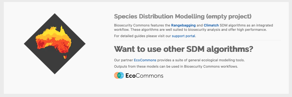
Biosecurity Commons integrated models

Biosecurity Commons provides direct integrated support for two profile (i.e. presence-only) models: Range-bagging and Climatch SDM algorithms commonly used for invasive species. These algorithms have seen recent applications to invasion biology and appear promising in the context of biosecurity. Part of their appeal is that no absences or background data are required – presence data are sufficient (Camac et al., 2020, Hill et al., 2022, Camac et al. 2024). This removes several subjective decisions required in the modelling process and focuses solely on the data commonly available for most threats – presence locations. Moreover, using Biosecurity Commons integrated models provides users with on-platform data cleaning routines powered by CoordinateCleaner (Zizka et al. 2019).

EcoCommons models

If users wish to utilise other SDM algorithms, they can directly access functionality available on our sister platform, EcoCommons. EcoCommons, a SDM specific platform, provides users with an additional 16 SDM algorithms spanning profile models (e.g. BIOCLIM), machine learning models (e.g. MaxEnt), statistical models (e.g. Generalised Additive Models) and geographic models (e.g. Convex and Voronoi hulls). EcoCommons provides functionality for forecasting species distributions under climate change. 

This guide focuses primarily on Biosecurity Commons integrated models, for details on how to use EcoCommons functionality, please see the BCCVL Modelling Wizard guide.

Step 2. Create a Species Distribution Model project using Biosecurity Commons integrated models

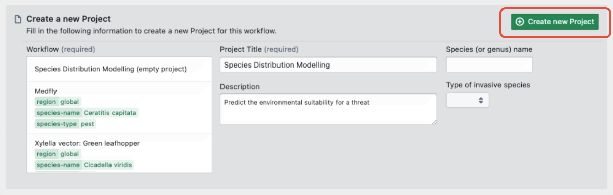
Select a workflow (see screenshot below) and then give your project a title. Users can also optionally provide additional descriptive details under the Description, Species name and Species type tabs. Project title is the only required field to be completed. Once details have been provided select the green “Create a new Project” button.

Step 3. Select your species occurrence data

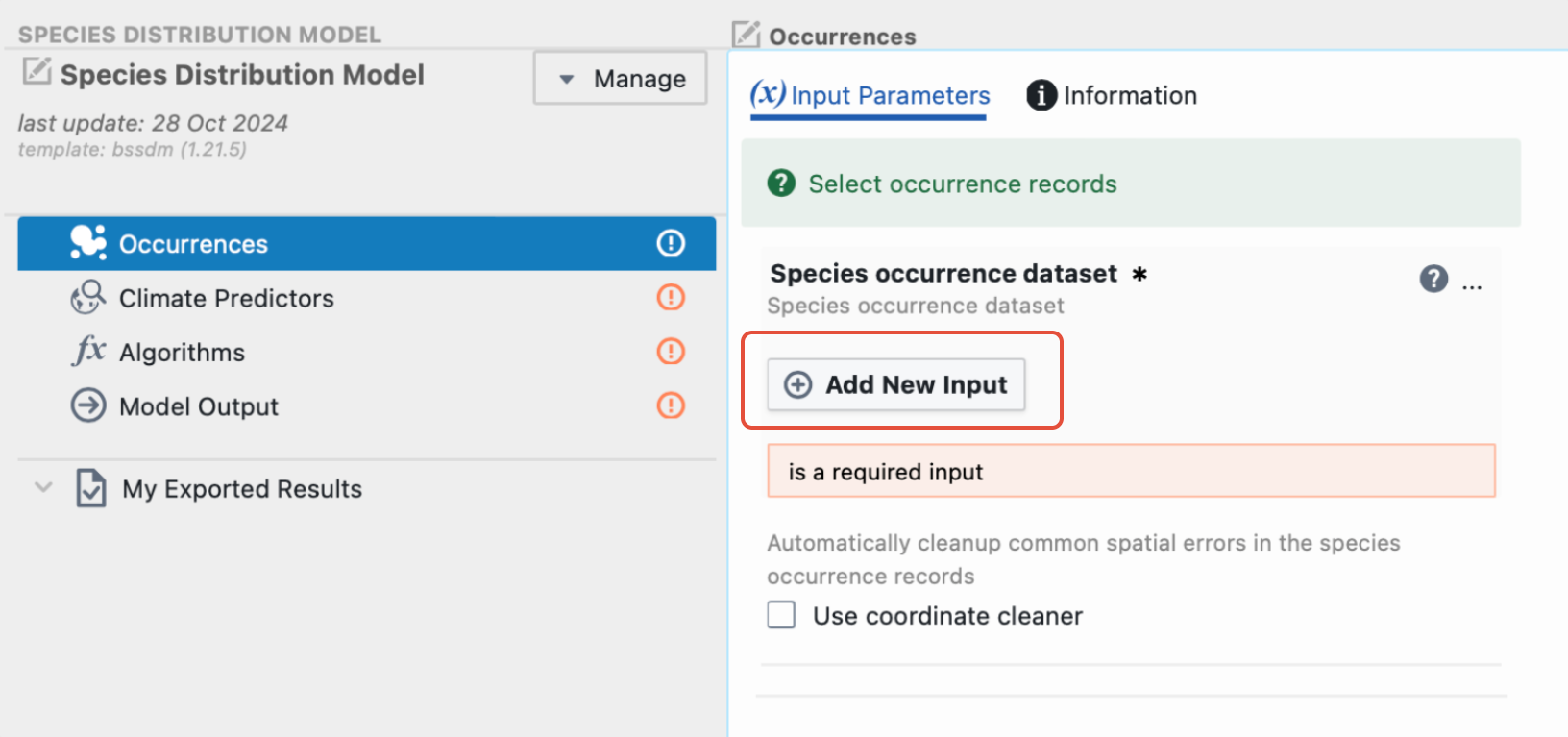
The two integrated species distribution models available on Biosecurity Commons are forms of correlative models. That is, they attempt to estimate environmental suitability as a function of spatial environmental data and known occurrence locations. As such, to fit these models, occurrence records are required. To add such data press “Add New Input”.

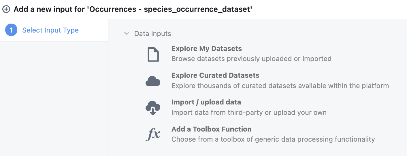
Users have four options to access or utilise occurrence records. They can:

• Search previously uploaded databases
• Search the curated database for pre-existing species-specific occurrences
• Upload their own georeferenced occurrence datasets
• Import data directly from third-party biodiversity databases, the Atlas of Living Australia (ALA), the Global Biodiversity Information Facility (GBIF), or for ocean species, Ocean Biogeographic Information System (OBIS).

1. Search your previously uploaded datasets

To search for occurrence records you’ve previously uploaded click “Explore My Datasets”. This will load up a window allowing users to search through datasets they have previously uploaded (see screenshot below).

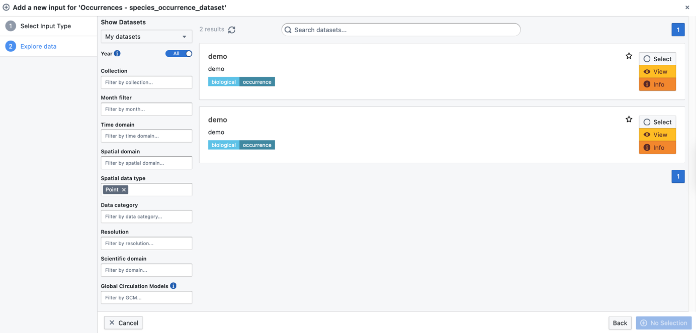
Users can then use the search to enter keywords to find the relevant dataset. Note, if users have many uploaded datasets, it is recommended they use the filtering options on the left to narrow down searches (see below for more details).

Once the relevant dataset is selected, simply click “Select” to the right of the dataset, and then click the blue “Add” button in the bottom right of the screen. 

2. Search for data on the Biosecurity Commons curated database

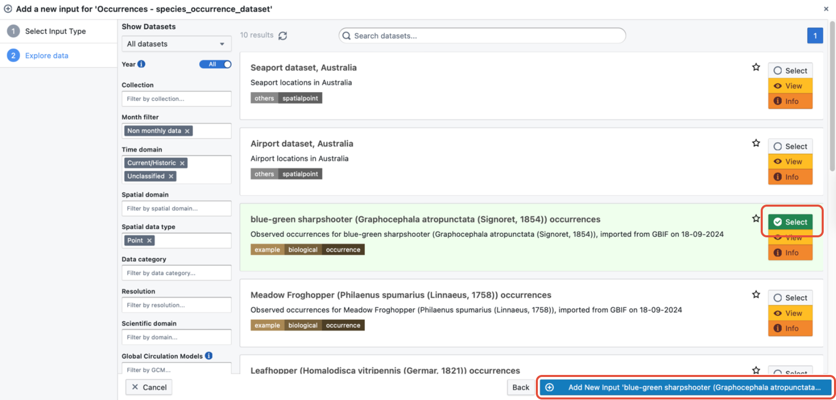
Users may wish to search through the curated datasets publicly available on Biosecurity Commons. To do this, select “Explore curated datasets”. This will load up a similar window to the screenshot above, however, this time users will be able to search the entire curated database.

Biosecurity Commons has thousands of datasets that users can access. As such, it can sometimes be challenging to find the dataset of interest. We strongly recommend using the filtering functionality to the left to navigate for appropriate datasets.
For occurrence records, we recommend users add the following filtering options:

Spatial data type = Point

Data category = Biological

These filtering options should narrow down the search to just occurrence point data that are available on the platform.

Once the relevant dataset is selected, simply click “Select” to the right of the dataset, and then click the blue “Add” button in the bottom right of the screen.

3. Upload own data

To upload your own data, click on import/upload data and follow these instructions.

4. Import occurrences directly from third-party

Biosecurity Commons also allows users to directly search and import occurrence data from Atlas of Living Australia (ALA), the Global Biodiversity Information Facility (GBIF) and the Ocean Biogeographic Information System (OBIS).

To do this, click Import/Upload data, then click “Import from third party” and then click “Species Occurrence”.

Users can select the database they wish to search from a dropdown menu. Species can then be searched using the search query. Note that both GBIF and OBIS require Latin species names. By contrast, ALA allows common names or Latin names. We strongly recommend searching using species Latin names, to minimise potential inconsistencies in naming.

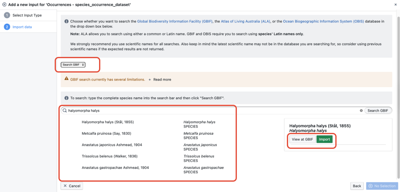
When the search is complete, users can select the relevant records they wish to import. 

For terrestrial exotic threats, GBIF is likely to be the primary database used to access global occurrence records. When a user finds appropriate records on GBIF, they can click the green “Import” button.

This will open a mini window that notifies the user of the number of records found, tells the users how many records (e.g. below there are 77,099 records).

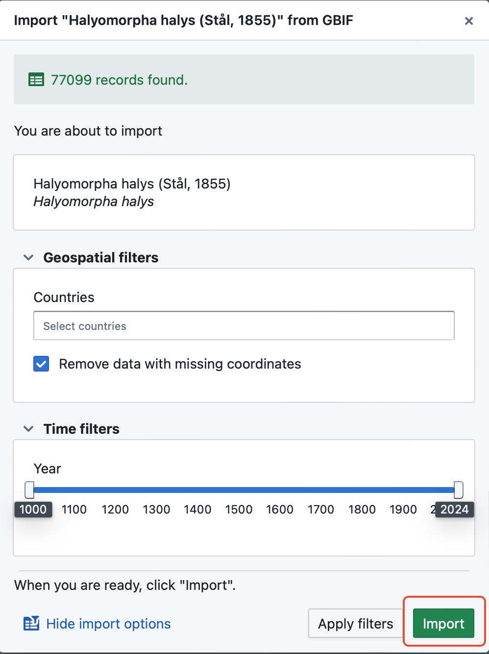
CAUTION: Users should take careful note of the record number, as GBIF currently has a cap of 100,000 records that can be directly imported onto the platform. This means that for species with more than 100,000 records, then records cannot be imported directly into the platform without some form of filtering the results in records falling below this number.

Irrespective of record number, we recommend users make appropriate use of the import Geospatial and Time filters. Specifically, we recommend users include countries where the pest has known to be established (i.e. attempt to remove transient records) and set the temporal period that is in alignment with period of the climate data (e.g. for WorldClim data, records post 1970). Once filters have been applied, click “Apply filters”. This will update the number of records to be imported. If less than 100,000 the platform will allow you to import. If greater than 100,000 we recommend sourcing the records directly from the GBIF website and then upload them to the platform.

Importing records directly from databases such as GBIF may take some time depending on the demand on their servers. Please be patient. 

Step 4. Clean your occurrences

Once an occurrence dataset has been selected, users have the option to clean these data using some inbuilt automated cleaning functionality available in the R package CoordinateCleaner. Specifically, Biosecurity Commons offers the following set of cleaning routines:

• Capital centroids: Remove records within a user-defined radius of capital centroids
• Country centroids: Remove records within a user-defined radius of a country centroid
• Equal: Remove records with equal latitude and longitude
• Institutions: Remove records within a user-defined radius from known biodiversity institutions (e.g. museums, herbariums, universities, botanic gardens)
• gbif: Remove records within 1 degree of GBIF headquarters in Copenhagen, Denmark.
• Zeros: Remove records with coordinates 0,0 or within a given radius of those coordinates
• Seas: Remove records with coordinates located in the ocean
  
  

To run these cleaning routines, simply click “Use coordinate cleaner”, then select the cleaning tests required, and if required, the test-specific radius.

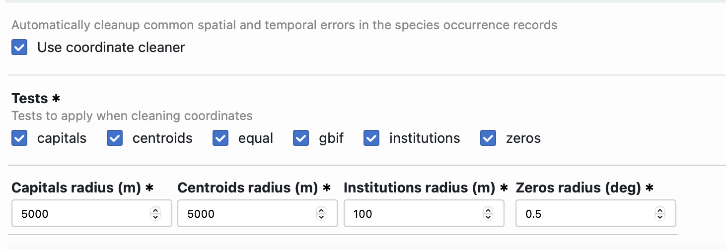
Once desired setting has been selected, click save at the bottom of the screen. 

You are now ready to move onto the climate predictor stage.

Step 5. Select climate predictors

Biosecurity Commons and its sister platform, EcoCommons, have a vast array of spatial datasets that can be used in species distribution models to infer suitability. To search this database, click “Add New Input”.

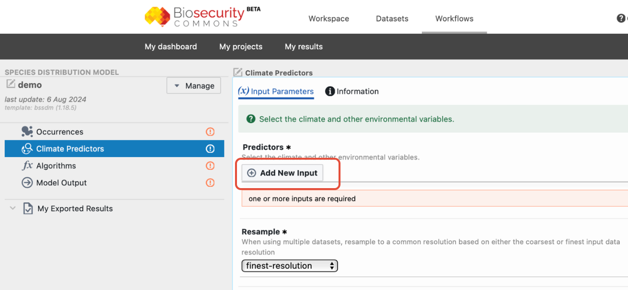
Then select “Explore curated datasets”.

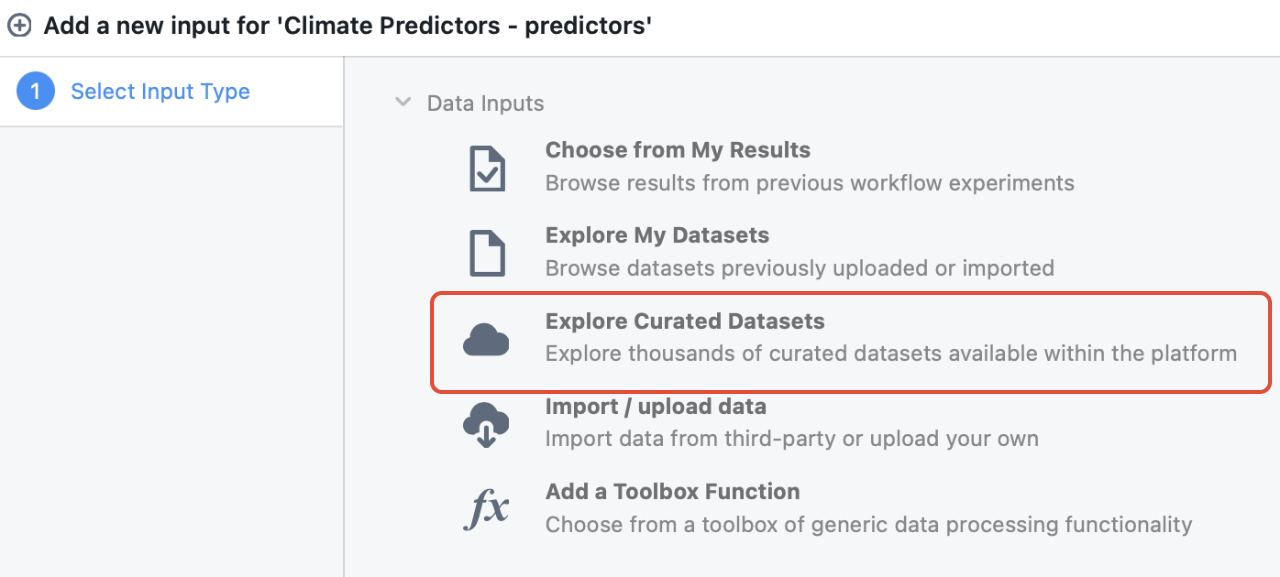
As the database contains over 50,000 datasets, we strongly recommend users utilise the filtering options to the left. Specifically, use the “Collection” filter to select the collection of data they wish to use.

For example, if a user wishes to use long-term average historical WorldClim BIOCLIM predictor data, we recommend that users first select “WorldClim-v2.1” in the “Collection” dropdown menu, ensure “Non monthly data” is specified in the Month filter, and “climate” is selected in the Data category. This should show the different WorldClim climate datasets available and their associated resolutions.

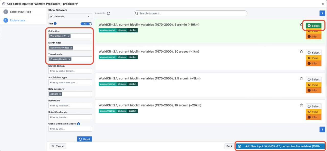
Once the relevant dataset is selected, simply click “Select” to the right of the dataset, and then click the blue “Add” button in the bottom right of the screen.

When you have selected your dataset, you will be able to choose from a list of climate and environmental variables (screenshot below). Select the layers that are related to your target species. 

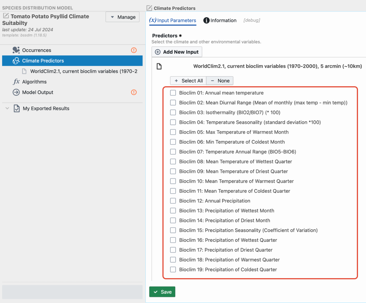
Note that users can select multiple datasets. If multiple datasets are selected and these are at different resolutions, the platform will automatically resample coarser resolution data inputs to the finest resolution selected – ensuring all input predictors are on a common resolution. 

Users can change this setting to resample finer resolution inputs to the coarsest resolution by changing “Resample” from “finest-resolution” to “coarsest-resolution.

When you are ready, click save and move to the algorithms stage.

Step 6. Choose your SDM algorithm

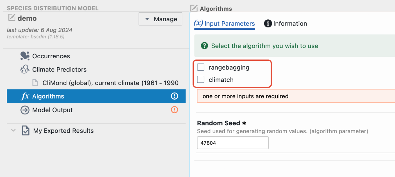
Users can choose either Range Bagging or Climatch, or both. Both models are profile models. That is, they only use presence records and do not use absence or background data in model fitting. These models simply describe the environmental conditions found across all the areas the species is known to occur.

Range Bagging

Range bagging is an algorithm that estimates the environmental limits of a species’ habitat by calculating convex hulls around environmental conditions at occurrence locations. Environments that fall within the hull are defined as suitable, whereas those that fall outside are considered unsuitable. This process is then repeated using random subsets of both occurrence records as well as available environmental covariates (e.g. annual rainfall, mean annual temperature, etc.). The number of covariates included in a replicate is defined by the user. Suitability is then defined for each raster cell as the proportion of replicates that define the location as suitable. For example, a suitability score of 0.1 would indicate only 10% of the estimated convex hulls ensembled deemed that location suitable. By contrast, a score of 0.9 would indicate that 90% of estimated convex hulls deemed that location climatically suitable.

Advantages: 

• Quick and easy profile method
• It is likely more robust than other profile methods due to 'bagging'
• Increasing evidence that algorithm performs well
• Ensemble of many models

Limitations:

• Only uses continuous predictor variables

Assumptions: 

• No assumptions are made about the distributions of the environmental variables.

Climatch

Climatch is a software tool developed by the Australian Bureau of Agricultural and Resource Economics and Sciences (ABARES). It assesses the climatic suitability of different geographic regions for a particular species by comparing the climate of a target region with the climate of regions where the species is already known to exist. Climatch analyses various climatic variables, such as temperature and precipitation, to predict the potential distribution of species, particularly invasive species, under current and future climate scenarios.

The software uses Euclidean distances to estimate climatic suitability. It calculates the Euclidean distance between the climate variables of the target region and those of the known regions. Smaller Euclidean distances indicate higher climatic similarity and thus higher suitability for the species. This method helps identify areas that are climatically suitable for the establishment and spread of species of interest, making Climatch a valuable tool for biosecurity, conservation planning, and managing invasive species risks.

Disclaimer: Please note that Biosecurity Commons implements the Climatch algorithm (Euclidean). As Biosecurity Commons allows users to input different climate predictor datasets, outputs will differ to those created using the official ABARES version. Details of the Climatch algorithm can be found in the Climatch manual Climatch (agriculture.gov.au).

Advantages:

• Quick and easy way to identify environmental space used by selected pests
• Only requires presence occurrence data included within a gridded study area
• Algorithm has been widely used in pest and weed biosecurity risk analyses
• Again, due to use of grid data on our platform the matching is not like the official

Climatch algorithm which compares target and source point locations

Limitations:

• Simple and less sophisticated approach than other SDM methods
• Does not allow model ensembling (i.e. is reliant on single model fit)
• Only uses continuous predictor variables

Users can select one or both algorithms. When both are selected, users will obtain two outputs, one per algorithm.

Once algorithms are selected, users may modify algorithm specific parameters (screenshot below). 

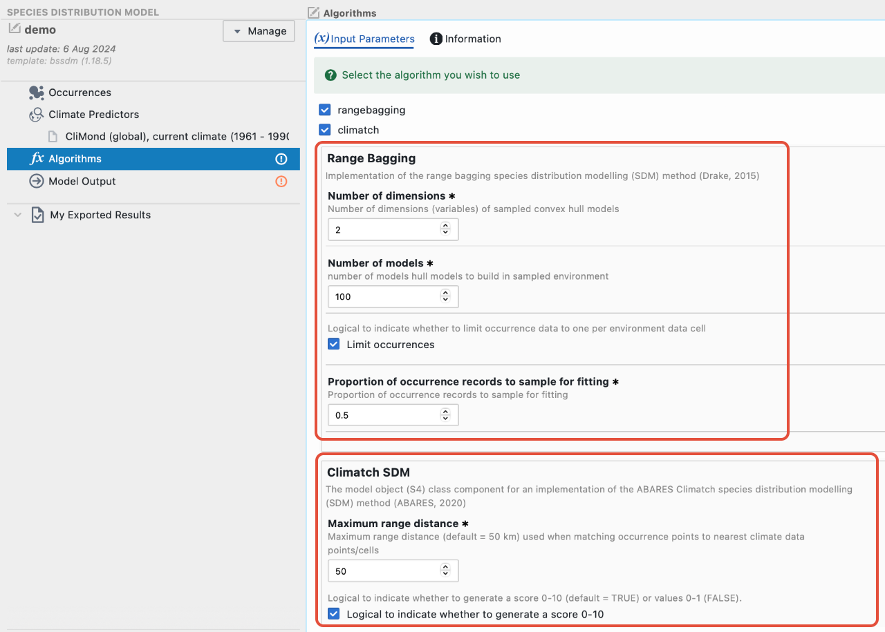
When you are ready, click save and move to model output. 

Step 7. Model outputs

If all required inputs have been specified, you will see the ‘ready to run’ message in green. 

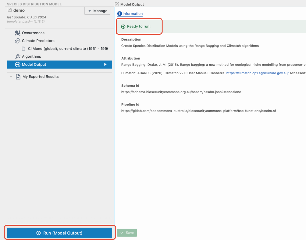
Click the blue ‘Run’ button in the bottom left to run your project. The output page will be updated as the job processes from “Created”, “Submitted”, “Started” and “Success”.

Once the models, or model, have finished, a green tick will appear next to Model Outputs. 

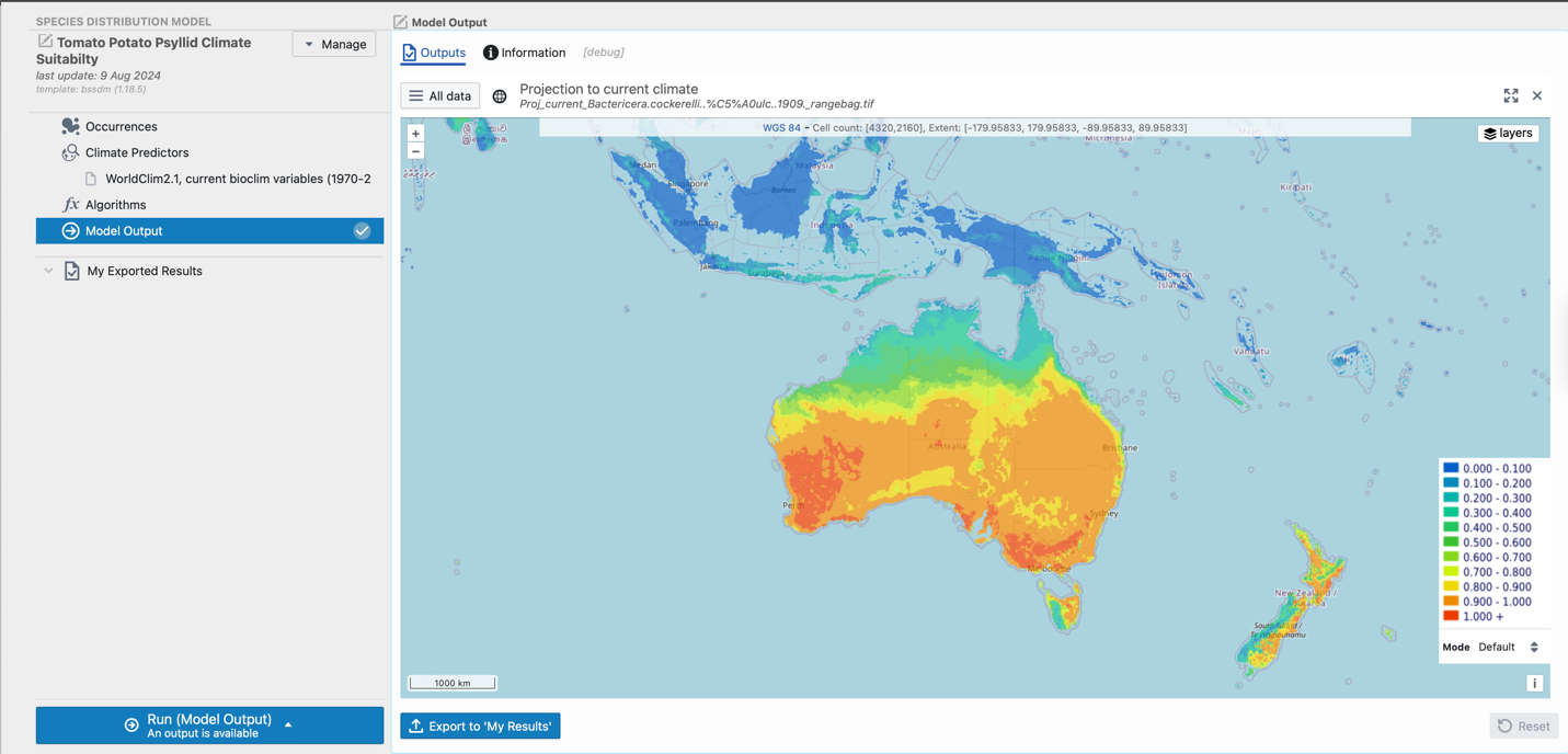
If users only selected one algorithm, the model output will automatically be displayed as a global heat map will be viewable in the interactive map pane. Users can zoom in or out of regions of interest. Interactive maps also allow users to change the type of legend displayed.

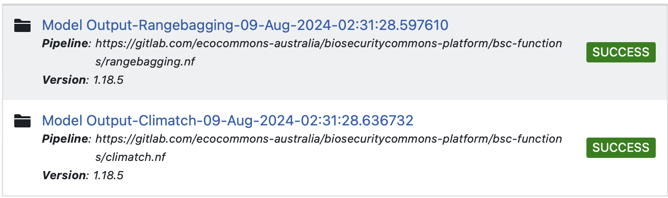
If users selected both algorithms, the heat map will not be automatically displayed. Rather, users need to select one of the two outputs.

And then select “View” on the file named “Projection to current climate”.

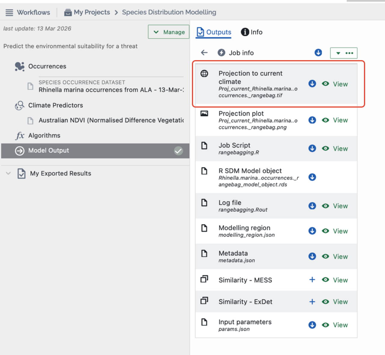
Note also, that model outputs also contain a variety of other outputs including:

• Projection plot: A .png global heat map of predicted suitability
• Job Script: A copy of the R script used to build the model
• R SDM Model object: A .rds file containing the model object
• Log file: A text data file containing processes, messages, and other details associated with model runs.
• Modelling region: A .json file defining the extent of the projections (this is always global extent)
• Metadata: A .json file containing the metadata required to run the model on Biosecurity Commons
• Input parameters: Input parameters required to run the Job Script. 
• MESS: GeoTiffs and pngs associated with the multivariate environmental similarity surface, indicating the degree of similarity between prediction-region and model-fitting conditions
• ExDet: GeoTiffs and pngs associated with the ExDet (Extrapolation Detection) score describing types and degree of environmental novelty

Users can download outputs by selecting the “Download” button.

Step 8. Exporting outputs for use in other workflows

Users may wish to export outputs for use in other projects or other workflows.

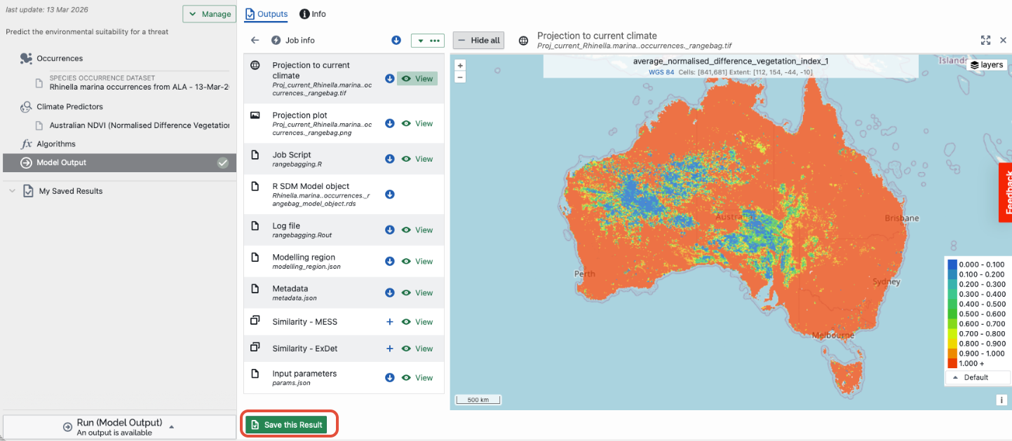
To do this, view the output of interest, and select in the bottom left corner of the interactive map “Save this Result”. This output will now be discoverable in the users “My results” database, which in turn, makes the layer available for use in other workflows.