Establishment Potential Mapping (Risk Mapping)

This article is focused on providing a more in-depth understanding of Establishment likelihood mapping. If you are interested in a step-by-step guide on how to use the Biosecurity Commons interface for establishment likelihood mapping please see our Risk Mapping Quick Start Guide.

Overview

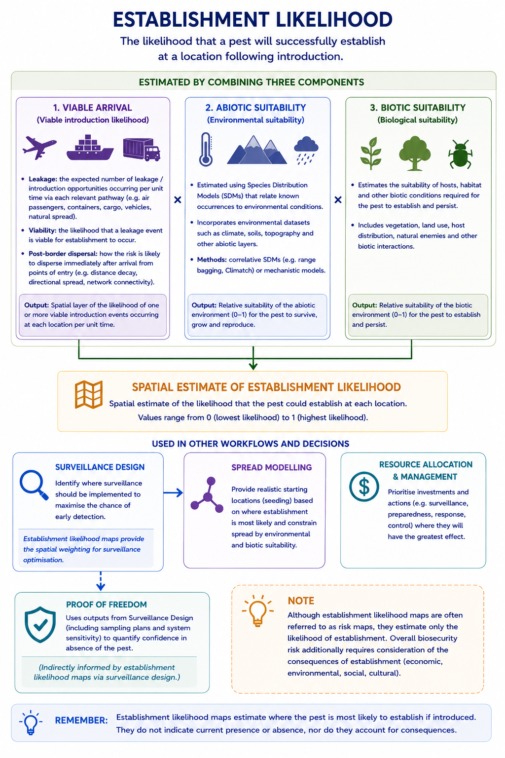
Although commonly referred to as the Risk Mapping workflow, the workflow estimates establishment likelihood rather than overall biosecurity risk. It identifies where an invasive species or biosecurity threat is most likely to arrive and establish by integrating viable arrival, abiotic suitability, and biotic suitability. Overall biosecurity risk can then be estimated by combining establishment likelihood with consequence information.

At its core, establishment likelihood mapping is based on three barriers to establishment. For a threat to establish, it must: (1) arrive, (2) encounter a suitable abiotic environment, and (3) have access to suitable biotic conditions (e.g. hosts or habitat). If any of these barriers are not met, establishment cannot occur (Figure 1).

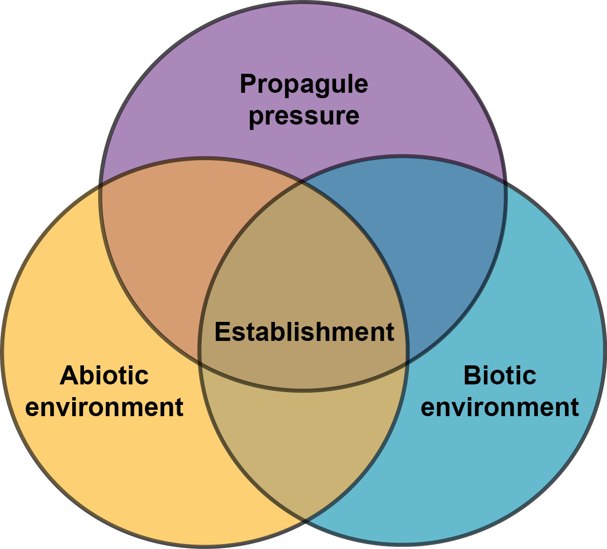
The three main elements governing the likelihood of threat establishment in an introduced region. (Camac et al. 2024).

How can establishment likelihood maps be used?

Maps of establishment likelihood are important decision-support tools in biosecurity. They help show where a pest, weed, or disease is most likely to establish if introduced, which in turn supports more targeted, transparent, and cost-effective decision-making (Camac et al. 2021; Camac et al. 2024).

• Prioritise surveillance for early detection
  These maps help identify the areas where a threat is most likely to establish, so surveillance can be focused where it is most likely to detect new incursions early.
• Target surveillance for one or many threats
  Maps can be used for a single threat, or combined across multiple threats to identify shared hotspots of establishment potential. This helps prioritise areas where surveillance may provide the greatest value across several threats at once (see Camac et al. 2021 for an example).
• Assess how well surveillance covers high-risk areas
  Establishment likelihood maps can be compared against existing or proposed surveillance designs to evaluate how much of the highest-priority area is being covered, including under different budget constraints (see Camac et al. 2020 for an example).
• Support inference about likelihood of absence
  Not detecting a threat does not prove it is absent. These maps can be combined with surveillance effort and surveillance sensitivity to estimate how likely it is that a threat is truly absent, while accounting for the fact that some areas are more suitable for establishment than others.
• Support proof-of-freedom and market access claims
  Because they improve inference about likely absence, establishment likelihood maps can help support pest freedom assessments that may be important for trade, certification, and market access.
• Initialise spread models more realistically
  Spread models need a starting point. Establishment likelihood maps provide a transparent way to place initial incursions in locations where establishment is actually plausible, rather than relying only on arbitrary or random starting locations.
• Improve invasion and spread simulations
  By accounting for propagule pressure and environmental suitability, these maps help create more realistic simulations of establishment and subsequent spread.
• Compare management strategies
  When used within spread modelling, establishment likelihood maps can help assess the likely benefits and costs of different pre-border, border, and post-border management options.
• Contribute to true risk maps
  Establishment likelihood is not the same as risk on its own. However, when combined with information on consequences such as economic, environmental, social, or cultural impacts, it can be used to develop spatial risk maps.
• Prioritise protection and mitigation activities
  Risk maps built from establishment likelihood and consequence layers can help identify where surveillance, control, or asset protection activities should be prioritised to reduce overall risk.

Choosing your study region

The study region defines the geographic extent, coordinate reference system (CRS), and spatial resolution used to generate the final risk map. Biosecurity Commons provides three alternative methods for defining the study region, depending on the type of analysis being undertaken.

Raster source (recommended for most workflows)

The Raster source is the default and recommended option for most risk mapping applications. It uses a raster template to define the study extent, coordinate system and output resolution. By default, this is a 1 km Australian Albers raster covering Australia, although users can select finer-resolution templates or supply their own raster template.

When using a raster source, users can define the study extent by:

• Using the full raster extent (e.g. all of Australia).
  Selecting one or more predefined regions, including Australian states and territories, Local Government Areas, Natural Resource Management regions, IBRA regions, river regions, drainage divisions and marine bioregions. Multiple regions can be combined and optional buffer distances applied to include surrounding areas.
• Drawing a custom extent directly on the interactive map using either a rectangular box or a freehand polygon.
• Providing an existing raster, either from previous workflow outputs, uploaded datasets, curated datasets or by uploading a GeoTIFF. This option is useful when the study region must align with an existing raster dataset or use a custom coordinate system and resolution.

Polygon source

The Polygon source allows users to define the study region using vector polygon boundaries rather than a raster template. Biosecurity Commons accepts either ESRI shape files or GeoPackages file types. This is useful when an existing polygon layer (e.g. management zones, administrative boundaries or property boundaries) defines the area of interest. The polygon is subsequently rasterised according to user defined resolution (default = 1km) and coordinate reference system (Default = World Cylindrical Equal Area) region template before the analysis is performed.

World region source

The World Region source provides a convenient way to define study regions outside Australia using predefined country boundaries. Users can select one or more countries by name, with the selected country boundaries automatically combined to define the analysis extent. This eliminates the need to manually draw or upload geographic boundaries. The combined extent is subsequently rasterised according to user defined resolution (default = 1km) and coordinate reference system (Default = World Cylindrical Equal Area) region template before the analysis is performed.

Importance of carefully defining the Coordinate Reference System and resolution

Irrespective of method used to define a region. It is critical that users carefully consider the spatial resolution and coordinate reference system used.

Coordinate Reference System

A Coordinate Reference System (CRS) defines how locations on the curved surface of the Earth are represented in a spatial dataset. Because the Earth is spherical, projecting it onto a flat map inevitably introduces distortion. Consequently, map projections are typically designed to preserve one spatial property—such as area, distance, shape (angles) or direction—while accepting distortion in the others. Some projections, such as the Australian Albers Equal Area projection, preserve area exactly while also keeping distance and shape distortions relatively small over their intended region.

For most biosecurity risk mapping applications, we recommend using the standard projected CRS adopted for your country or jurisdiction. In many cases, this will be an equal-area projection, which ensures that raster cells represent consistent ground areas and avoids systematic bias when comparing, combining or summarising spatial risk across a landscape. However, the optimal CRS depends on the intended use of the risk map, as different projections prioritise different spatial properties, such as preserving area, distance, shape or direction.

Biosecurity Commons provides a selection of commonly used equal-area projections for several countries, and users may also specify any CRS using its EPSG code. If you are unsure which CRS is most appropriate for your study region, we recommend consulting https://epsg.io/ or your national mapping authority for guidance. If a suitable regional projection is unavailable, World Cylindrical Equal Area (EPSG:6933) provides a good global equal-area alternative.

Selecting an Appropriate Resolution

The spatial resolution determines the size of each raster cell used to represent the study region and therefore the level of spatial detail in the resulting risk map. Selecting an appropriate resolution is an important decision, as it should reflect both the management objective and the spatial scale at which the underlying processes operate. For example, broad-scale national prioritisation may only require a 1 km or coarser resolution, whereas local surveillance planning or property-level decision-making may warrant finer resolutions.

Increasing the spatial resolution does not necessarily improve the quality or accuracy of a risk map. Finer resolutions substantially increase computational requirements and may imply a level of precision that is not supported by the underlying datasets or ecological processes. In general, users should select the coarsest resolution that adequately addresses their management objective while remaining consistent with the resolution and uncertainty of the available input data.

Abiotic Suitability

Abiotic suitability describes whether the physical environment—most commonly climate—is suitable for a species to survive and reproduce. It is commonly estimated using species distribution modelling (SDM) approaches, which link observed occurrences or known physiological limits of a species to environmental variables (e.g. temperature, rainfall), and project these relationships across landscapes to identify areas of suitable conditions.

Biosecurity Commons currently provides two SDM algorithms for estimating abiotic suitability:

• Range Bagging (Drake 2015)– a presence-only ensemble envelope approach
• Climatch (Crombie et al. 2008)– a climate similarity-based method

These approaches are particularly well suited to invasive species applications, where reliable absence data are rarely available, distributions are still expanding, and species may not yet be in equilibrium with their environment.

Presence-only and climate similarity methods reduce the need for strong modelling assumptions, while still providing robust and interpretable estimates of potential climatic suitability.

They are intentionally lightweight and accessible, making them well suited to rapid assessments, screening analyses, and operational decision-making, where transparency, reproducibility, and speed are critical. For more details about these methods please see the Biosecurity Commons SDM support article.

However, if users wish to apply alternative modelling approaches (e.g. MaxEnt, Boosted Regression Trees, Random Forests, or other machine learning methods), these can be run externally and imported into Biosecurity Commons. This can be done either by developing models locally and or on EcoCommons and uploading/importing model results into Biosecurity Commons.

EcoCommons is a national, cloud-based ecological modelling platform that provides access to a wide range of advanced species distribution modelling (SDM) tools. It leverages the same curated environmental datasets available in Biosecurity Commons (e.g. WorldClim, soil, and land use layers), and offers reproducible SDM workflows for model training, evaluation, and projection.

For guidance on using EcoCommons, see:

• EcoCommons Modelling Wizard Guide
• EcoCommons Support Portal

Outputs from EcoCommons (e.g. GeoTIFF suitability layers) can be uploaded directly into Biosecurity Commons and used within the risk mapping workflow.

Biotic Suitability

Biotic suitability reflects whether the living components of an environment can support the establishment and persistence of a threat. This includes the availability of required hosts, food sources, and habitat structure, as well as interactions with other species such as competitors, predators, or facilitators. In many cases, biotic suitability acts as a key constraint on establishment even where climatic conditions are favourable, as a species must be able to locate and utilise suitable resources to survive and reproduce.

In practice, biotic suitability is often approximated using spatial datasets that describe habitat or resource availability. Common data sources include detailed land use and vegetation maps, distributions of host species or commodities, and remotely sensed indicators such as vegetation cover or greenness. At finer spatial scales, country/region-specific datasets (e.g. high-resolution land use classifications, agricultural production layers, or host crop distributions) are particularly valuable, as they can capture the heterogeneity in habitat and resource availability that is critical for establishment.

Biosecurity Commons has a wealth of datasets that can be used to inform biotic suitability (especially in the Australian context). Examine our curated datasets here.

Use Function

The Use Function option allows users to generate a new biotic suitability layer by combining one or more existing raster datasets using a mathematical function. This provides a flexible way to derive suitability from environmental variables such as host availability, habitat type, vegetation, land use or food resources, rather than relying on a pre-existing suitability map. It is particularly useful when biotic suitability depends on multiple factors or when users wish to construct custom suitability layers from existing spatial datasets.

Three combination functions are available:

• Product (prod) – Multiplies the input layers together. This is appropriate when all conditions must be met for establishment to occur. For example, a pest may require both a suitable host and suitable nesting habitat. A low suitability in any input layer reduces the overall suitability, making this the recommended option when the inputs represent sequential or limiting ecological requirements.
• Sum (sum) – Adds the values from each input layer. This is most appropriate when the inputs represent independent contributions to suitability that accumulate across the landscape, such as the abundance of multiple host species or habitat resources. Users should ensure that the resulting values remain on an appropriate scale for subsequent analyses.
• Union (union) – Combines probability layers using the equation 1 − ∏(1 − x), representing the probability that at least one of the input conditions is suitable. This option should only be used when the input layers represent probabilities and the presence of any one condition is sufficient for establishment. For example, if a pest can establish on any one of several alternative host species, the union function provides an appropriate estimate of overall biotic suitability.

Recommendation: In most ecological applications, the Product function is the preferred option because establishment typically requires multiple environmental constraints to be satisfied simultaneously. The Union function is recommended when combining probabilities associated with alternative hosts or habitats, while Sum is best reserved for combining additive indices or measures of resource availability rather than probabilities.

Binarize

The Binarize checkbox converts the combined output into a binary raster. Cells with values greater than zero are assigned a value of 1 (suitable/present), while cells with a value of zero remain 0 (unsuitable/absent). This is useful when users are interested only in whether suitable conditions exist, rather than the relative magnitude of suitability.

Pest Arrival and Propagule Pressure

Establishment of an invasive species requires not only suitable environmental conditions, but also the arrival of viable individuals (Hulme 2009). This is commonly described as propagule pressure—the likelihood or expected number of contamination events entering a region. Propagule pressure is widely recognised as a key determinant of establishment risk, as higher rates of arrival increase the probability that at least one introduction event results in a self-sustaining population.

In biosecurity systems, propagule pressure is driven by pathways of entry (e.g. passengers, cargo, mail, or natural dispersal), and reflects both how often contamination events occur and whether those events are capable of establishing. To capture this, Biosecurity Commons represents pest arrival using two complementary components: leakage limits and viability limits.

Leakage and Viability Limits

Leakage limits describe the expected number of contamination events that bypass border controls for a given pathway. These are typically expressed as lower and upper bounds on the number of post-border leakage events per year, reflecting uncertainty in pathway risk and incorporating information from interception data (Camac et al. 2024a), pathway volume, and expert judgement (Hemming et al. 2017).

Viability limits describe the probability that a given contamination event is capable of establishing. This accounts for factors such as survival along the pathway, the size and condition of the introduced population, and whether individuals arrive in a state that allows successful establishment. Again, these limits can be informed by interception data (that assesses survivability and population sizes) and can be supplemented by expert elicitation (Hemming et al. 2017).

Within Biosecurity Commons, users specify both lower and upper bounds for leakage and viability parameters, along with an associated confidence level. This allows uncertainty in pathway risk to be explicitly represented, rather than relying on single point estimates. By defining plausible ranges and confidence, the platform can propagate this uncertainty through to estimates of arrival likelihood and establishment risk.

Together, these parameters separate two critical components of pest arrival risk:

• Leakage – how often contaminated material enters the system
• Viability – how likely those events are to result in a viable introduction

This distinction is important because not all pathways that contribute to leakage necessarily contribute equally to establishment risk. For example, some pathways may have relatively high leakage rates but low viability due to high mortality or small propagule sizes, resulting in a low overall contribution to establishment potential. Conversely, pathways with lower leakage but higher viability may represent a greater risk of successful establishment.

Dispersing Pathway-Specific Risk

Once propagule pressure has been estimated for each pathway, risk must be spatially distributed across the landscape. This is achieved by allocating pathway-specific arrival likelihoods to locations based on spatial weighting functions that reflect how goods, people, or natural dispersal processes move post-entry.

Distributing pathway-specific risk requires approximating how contaminated carriers (e.g. people, goods, or natural vectors) move after entering a region. Ideally, these movements would be informed by detailed empirical tracking data; however, such data are rarely available at the spatial and temporal scales required. As a result, pathway dispersal is typically approximated using a combination of available datasets and simple, interpretable weighting functions.

At a minimum, pathway analyses require information on: (1) the volume of pathway carriers (e.g. passengers, cargo, or mail), (2) the likelihood that a carrier contains a viable threat, (3) the probability that contaminated carriers bypass border controls, and (4) how those carriers disperse post-border. The final component—post-border dispersal—is often the most uncertain, and is typically approximated using spatial proxies that reflect human movement, demand, or environmental processes. 

Common data sources and assumptions used to distribute pathway risk include:

• Population density – used to approximate where people, goods, and services are concentrated, and therefore where many pathways (e.g. returning residents, mail, imported goods) are likely to terminate.
• Tourist accommodation density – used to represent where international visitors are likely to congregate shortly after arrival.
• Distance from ports or airports – incorporated via distance-decay functions to reflect decreasing likelihood of arrival with increasing distance from points of entry.
• Transport and trade data – such as container destination data or commodity flow information, where available, to more directly represent movement pathways.
• Land use and agricultural activity – used to distribute pathways linked to farming systems (e.g. fertiliser, machinery), often coupled with measures such as farm density or production intensity.

In practice, these datasets are combined into pathway-specific weighting functions that describe how arriving pathway units are distributed across the landscape. These functions allocate the proportion of arrivals expected at each location based on plausible movement patterns. For example, passenger-based pathways may be modelled using a combination of distance from airports and population density, while tourism-related pathways may combine distance decay with accommodation density. More broadly, these weighting functions are designed to reflect realistic post-entry behaviour, such as the tendency for goods to move toward areas of high demand, or for travellers to remain close to entry points shortly after arrival. There is empirical support for the use of such proxies, with studies consistently showing that factors such as land use, road density, and human population density are strongly associated with first detections of exotic threats, even after accounting for potential survey bias (e.g. Dodd et al. 2016).

Although simplified, these approaches provide a transparent and flexible way to approximate post-border dispersal, enabling the construction of spatially explicit propagule pressure maps that can be integrated with abiotic and biotic suitability to estimate overall establishment likelihood.

Important Note: Biosecurity Commons allows users to use any raster layer to spatially distribute pathway risk. It is not necessary to transform the data into a proportional risk layer before uploading, as the platform performs this conversion automatically. For example, users can upload a raster of human population counts, and Biosecurity Commons will convert it into a proportional layer representing the fraction of the total population located within each cell of the user-defined study region.

Mathematical Framework

The workflow models arrival and establishment as a sequence of probabilistic processes, explicitly incorporating uncertainty in both pathway leakage and viability. Users provide lower and upper bounds for each parameter, and these bounds are used to define probability distributions that are then propagated through the workflow.

Leakage (Entry Events)

Plain language: Users specify lower and upper bounds for the annual number of leakage events for pathway k. These bounds are used to estimate the centre and spread of a log-normal distribution for the expected annual entry rate, λ_k. A Poisson distribution is then used to simulate the actual number of entry events in a given year. Note that the 1.96 refers the number of standard deviations that associated with the level of confidence set. In this case, we assume the default confidence level of 0.95.

What this is doing: Rather than assuming a single fixed number of arrivals, the model treats leakage as uncertain. The lower and upper bounds define a plausible range for annual entry events, and the simulation captures year-to-year variability around that uncertain rate.

Viability (Successful Introductions)

Plain language: Users also specify lower and upper bounds for the probability that a leakage event is viable. These bounds are converted onto the logit scale to define a distribution for pathway viability, p_k. The number of viable introductions is then modelled as a binomial draw from the total number of entry events. Note that the 1.96 refers the number of standard deviations that associated with the level of confidence set. In this case, we assume the default confidence level of 0.95.

What this is doing: This separates how often contaminated material enters the system from how often those entry events are actually capable of establishing. It allows the model to account for uncertainty in pathway survival, propagule size, and other biological constraints on establishment.

Spatial Allocation

Plain language: The viable introductions for pathway k are then distributed across space using a pathway-specific weight, w_i,k, which describes the proportion of pathway units expected to arrive at location i. This equation calculates the probability that at least one viable introduction arrives in cell i.

What this is doing: Some cells are more likely to receive arrivals than others because of where people travel, where goods are moved, or how pathways disperse after entry. The weighting layer allocates arrival pressure spatially, and the equation converts that into the probability of one or more viable arrivals reaching a cell.

Combining Pathways

Plain language: Multiple pathways may contribute to arrival risk at the same location. This equation combines the pathway-specific probabilities to estimate the probability that one or more viable introductions occur in cell i across all pathways.

What this is doing: Even if each pathway is individually unlikely, the combined arrival probability can become much higher when several independent pathways contribute risk to the same location.

Final Establishment

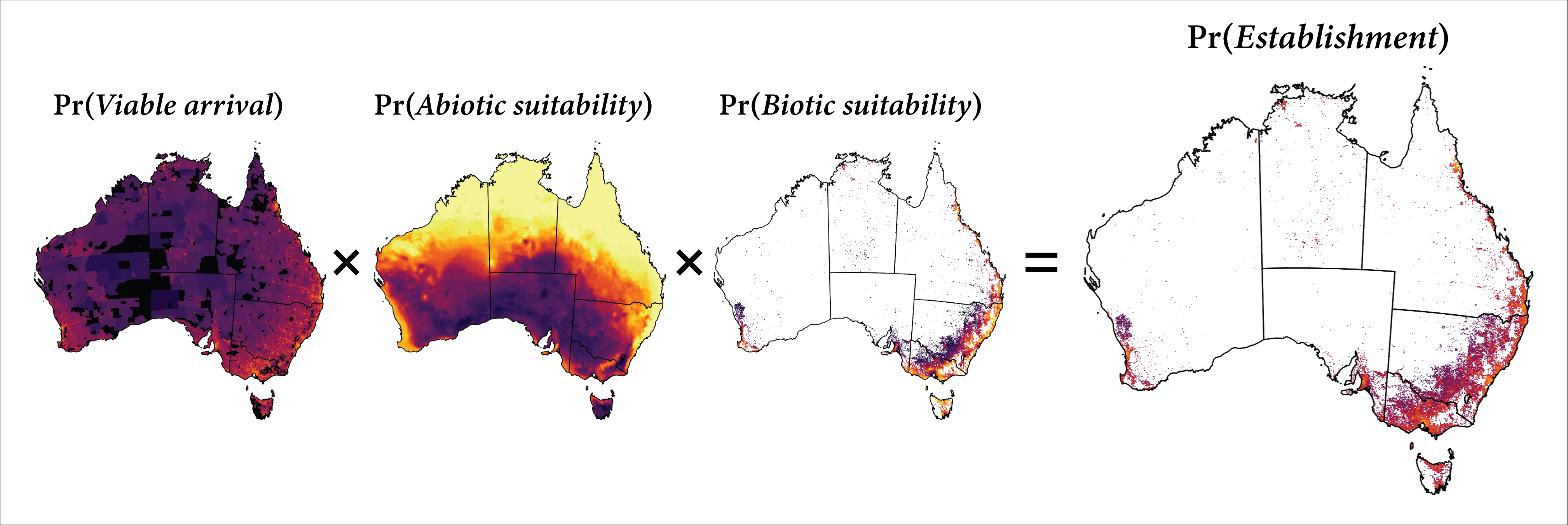
Plain language: Establishment at a location depends on three things aligning: viable arrival, suitable abiotic conditions, and suitable biotic conditions. Note that in this context, the product of biotic suitability and abiotic suitability is commonly referred to as the "threat suitability layer".

What this is doing: This final step integrates the three core barriers to establishment into a single estimate of establishment likelihood. A location can only have high establishment potential when arrival pressure is non-negligible and both the physical and living environment are suitable.

For more comprehensive descriptions of this method please consult Camac et al. (2020) and the extension report Camac at al. (2021)

Common Mistakes and Best Practice

Confusing establishment likelihood with risk

Establishment likelihood maps are often informally referred to as risk maps, but they do not represent biosecurity risk on their own. They estimate where a pest is most likely to establish if introduced, based on viable arrival, abiotic suitability, and biotic suitability. They do not account for the consequences of establishment, such as economic losses, environmental impacts, social effects, or cultural values.

As a result, two locations may have similar establishment likelihoods but very different overall risks if the potential consequences differ substantially. Likewise, an area with relatively low establishment likelihood may still warrant high priority if the consequences of establishment would be severe.

Best practice: Interpret workflow outputs as establishment likelihood maps, not risk maps. Where overall biosecurity risk is required, combine establishment likelihood with appropriate consequence layers (e.g. economic, environmental, social, or cultural impact) to produce a spatial risk assessment.

Treating leakage and viability inputs as relative weights across pathways

Users may sometimes specify leakage rates and viability bounds as relative weights to differentiate between pathways (e.g. “pathway A is twice as important as pathway B”), rather than as quantities grounded in real-world meaning.

While the platform can accommodate relative differences (e.g. by specifying proportional differences in leakage bounds or in the implied probability of one or more entry events), doing so means the outputs are no longer calibrated to real-world probabilities of establishment.

When combining multiple pathways, the model aggregates these inputs to estimate the probability of one or more entry events occurring across all pathways (i.e. the complement of no entry across pathways). However, if the underlying inputs are specified only in relative terms, this combined probability reflects a relative measure of entry pressure, not an absolute probability of introduction.

As a result, outputs should be interpreted as relative likelihoods rather than true probabilities, which can be misleading—particularly when comparing scenarios, jurisdictions, or when using outputs in downstream analyses such as surveillance design or risk estimation.

Best practice: Where possible, specify leakage rate bounds as realistic estimates of the expected number of contaminated units entering per year for each pathway. If using inputs that are relative to other pathways, restrict this to exploratory analyses and clearly communicate when outputs are relative rather than absolute.

Not aligning biology with biotic layers

Biotic suitability is often approximated using proxy datasets such as land use, vegetation type, or host distributions. However, these layers may not accurately represent the biology of the species of interest. For example, using broad land use classes may fail to capture specific host species, phenological requirements, or microhabitat conditions required for establishment.

Best practice: Select or derive biotic layers that closely reflect the species’ ecology (e.g. known host distributions rather than general vegetation classes), and ensure assumptions are transparent and defensible.

Using unvalidated occurrence data (including transient records)

Users may fit species distribution models (SDMs) without first checking occurrence records for common data issues or whether records represent established populations. Occurrence datasets (e.g. GBIF) can contain errors such as incorrect coordinates, duplicates, records located at country centroids or institutions, and observations from transient or intercepted individuals rather than established populations. Including these records can bias models by incorrectly characterising the environmental conditions under which a species can persist, leading to overestimation or misplacement of suitable areas.

Best practice: Use tools such as CoordinateCleaner (Zizka et al. 2019 – available on the platform) to systematically remove common spatial errors (e.g. country centroids, institutions, zero coordinates, and duplicates). In addition, where possible, restrict occurrence records to regions where the species is known to be established, based on literature, pest distribution databases, or expert knowledge.

Ignoring extrapolation diagnostics

Species distribution model (SDM) predictions in novel environmental space may be unreliable, particularly when transferring models across regions or under future climate scenarios.

Best practice: Use MESS and ExDet outputs to identify where predictions involve extrapolation, and interpret these areas with caution.

Failing to align temporal scales

Mismatches between the timing of occurrence records and environmental covariates can introduce bias. For example, fitting SDMs using occurrence records from 2000–2024 with climate data representing 1970–2000 conditions may misrepresent current suitability.

Best practice: Ensure occurrence data aligns with the temporal extent of environmental covariates (e.g. use post-1970 records for WorldClim 2.1).

Over-interpreting resolution

Fine-resolution outputs can imply a level of precision that is not supported by the underlying data or assumptions, particularly when inputs are coarse or highly uncertain.

Best practice: Match interpretation to the scale and quality of input data, and avoid drawing fine-scale conclusions from coarse or uncertain inputs.

Want to use our R package?

Biosecurity Commons is powered by a number of specially built R packages. If you would like to use our risk mapping method in R please visit our bsrmap GitHub page

References

• Camac, J. S., Baumgartner, J. B., Robinson, A., & Elith, J. (2020). Developing pragmatic maps of establishment likelihood for plant pests.
• Camac, J. S., Baumgartner, J. B., Hester, S., Subasinghe, R., & Collins, S. (2021). Using edmaps & Zonation to inform multi-pest early detection surveillance designs.
• Camac, J. S. (2024). Detect: Designing post-border surveillance schemes. In Hester et al. (Eds.), Biosecurity: A Systems Perspective. Taylor & Francis.
• Camac, J.S., Cantele, M., Pham, V.H., Li, C., Robinson, A., Kompas, T. (2024a) Forecasting trade and biosecurity risk under climate change. CEBRA project 21B. Technical

  Report for the Department of Agriculture, Fisheries and Forestry.

• Crombie, J., Brown, L., Lizzio, J., & Hood, G. (2008). Climatch user manual.
• Drake, J.M. (2015) Range bagging: a new method for ecological niche modelling from presence-only data. J R Soc Interface; 12 (107): 20150086.
• Dodd, A.J., McCarthy, M.A., Ainsworth, N. & Burgman MA. (2016) Identifying hotspots of alien plant naturalisation in Australia: approaches and predictions. Biol Invasions 18, 631–645.
• Elith, J., Kearney, M., & Phillips, S. (2010). The art of modelling range-shifting species.
• Hemming V, Burgman MA, Hanea AM, McBride MF, Wintle BC. (2018) A practical guide to structured expert elicitation using the IDEA protocol. Methods Ecol Evol; 9:169–180.
• Hulme, P.E. (2009) Trade, transport and trouble: managing invasive species pathways in an era of globalization. Journal of Applied Ecology, 46: 10-18.