- Overview
- Scope of the workflow
- Types of Surveillance
- Representing Surveillance Effort
- Representing the Surveillance Environment
- Occurrence Probability (or Relative Weight)
- Detection Parameters
- Surveillance Allocation
- Optimisation objectives
- Operational constraints
- Common Mistakes
- Want to use our R package?
- References
This article is focused on providing a more in-depth understanding of the optimal surveillance design workflow. If you are interested in a step-by-step guide on how to use the Biosecurity Commons interface for optimal surveillance design please see our Surveillance Design Quick Start Guide.
Overview
Surveillance is one of the most important tools available to biosecurity practitioners for supporting area freedom for market access, early detection of new incursions, incursion delimitation, and monitoring the success of eradication or containment programs (Camac 2024). However, surveillance resources are always limited.
Decisions about where to place traps, conduct surveys, or invest monitoring effort therefore need to maximise the information gained from every dollar spent.
The optimal design of a surveillance program depends not only on the surveillance objective, but also on the spatial distribution of biosecurity risk, the effectiveness of the surveillance method, and the operational resources available (Camac 2024). A surveillance network designed to detect a new incursion as early as possible will often differ from one designed to delimit an established outbreak or demonstrate that a pest is absent from an area. Understanding the purpose of surveillance is therefore the first step in determining where surveillance resources should be deployed.
Biosecurity Commons supports four common post-border surveillance objectives:
- Area freedom (market access) — provide evidence that a pest or disease is absent from a region or production area to support domestic or international market access.
- Early detection — maximise the likelihood of detecting a new incursion while populations remain small and geographically restricted, increasing the chance of successful eradication.
- Incursion delimitation — determine the geographic extent of a newly detected outbreak so that response activities can be targeted effectively.
- Monitoring and proof of freedom — evaluate the effectiveness of eradication or containment programs and provide evidence that a pest has been successfully eradicated or remains contained.
The Surveillance Design workflow supports these objectives by helping users evaluate existing surveillance networks or design new ones. Central to both applications is system-wide sensitivity—the probability that the surveillance system detects at least one incursion somewhere within the study region, assuming the invasive species is present. Unlike the sensitivity of an individual trap or survey, system-wide sensitivity measures the performance of the surveillance network as a whole. Existing system-wide sensitivities can also be exported directly into the Proof of Freedom workflow to quantify confidence that a pest is absent following zero detections.
Accordingly, the workflow provides two complementary capabilities:
- Evaluate existing surveillance networks by calculating the spatial detection probabilities and overall system-wide sensitivity of a surveillance design. This allows practitioners to quantify the effectiveness of current surveillance programs, compare alternative surveillance strategies, or assess changes in surveillance performance over time.
- Optimise surveillance resource allocation by identifying where surveillance should be deployed to best achieve a specified management objective. Depending on the decision context, optimisation can:
- maximise system-wide sensitivity (the probability of detecting at least one incursion somewhere within the surveillance region), making it well suited to early detection;
- maximise the expected number of detections, making it well suited to incursion delimitation, where accurately defining the extent of an outbreak is the primary objective;
- minimise the combined surveillance and incursion management costs;
- maximise net monetary savings (avoided damages minus surveillance costs); or
- maximise a user-defined non-monetary benefit, such as protecting biodiversity, species richness, or other high-value assets.
Optimisation can also be performed subject to practical constraints, including available budget, desired system-wide sensitivity, minimum surveillance allocations, and fixed deployment costs. The methodology behind the optimisation implemented on Biosecurity Commons is a generalised version of methods produced by Cannon (2009), Hauser & McCarthy (2009), McCarthy et al. (2010), Moore et al. (2016), & Anderson et al. (2017).
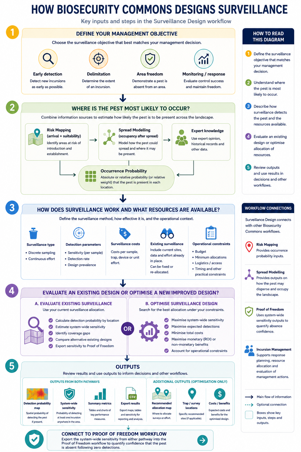
Schematic of Biosecurity Commons Surveillance Design Workflow.
Scope of the workflow
The Surveillance Design workflow is designed to determine where surveillance resources should be allocated to best achieve a specified surveillance objective. It is not intended to determine how frequently locations should be resampled or how much surveillance is required at an individual location to achieve a desired level of confidence that a pest is absent. These questions are addressed by the Proof of Freedom workflow, which uses surveillance sensitivity to estimate confidence of pest absence following zero detections. Together, the two workflows support complementary aspects of surveillance planning: Surveillance Design determines the optimal spatial allocation of surveillance, while Proof of Freedom quantifies confidence in pest absence based on the surveillance undertaken.
Types of Surveillance
Post-border biosecurity surveillance can be broadly classified into three complementary approaches: active, general, and passive surveillance (Camac 2024). These approaches differ in who undertakes the surveillance, how structured the surveillance effort is, and the confidence that can be placed in the resulting data. In practice, effective biosecurity systems typically rely on a combination of all three approaches.
Active surveillance
Active surveillance is the deliberate and coordinated deployment of surveillance specifically designed to detect a target pest or disease. Examples include routine trapping programs, targeted field surveys, diagnostic testing, detector dogs, and environmental DNA (eDNA) sampling. Because surveillance effort, detection methods, and survey protocols are well defined, active surveillance provides the most reliable evidence for early detection, outbreak delimitation, area freedom, and proof of freedom following eradication. The trade-off is that active surveillance is typically the most resource-intensive and costly form of surveillance.
General surveillance
General surveillance is undertaken by stakeholders such as farmers, veterinarians, agronomists, park rangers, industry groups, researchers, and citizen scientists as part of their routine activities. It provides broad geographic coverage at relatively low cost and has contributed to many first detections of invasive species. However, surveillance effort and detection reliability are often unknown or highly variable, making general surveillance less suitable for formally demonstrating pest absence without additional supporting evidence.
Passive surveillance
Passive surveillance relies on the chance detection and reporting of pests or diseases by members of the public. Reports may be submitted through biosecurity hotlines, citizen science platforms, or other reporting systems. Passive surveillance can provide valuable early detections, particularly for conspicuous species, but reporting effort is unstructured and detection probability is generally unknown. Consequently, passive surveillance is best viewed as a complementary source of intelligence rather than a stand-alone surveillance system.
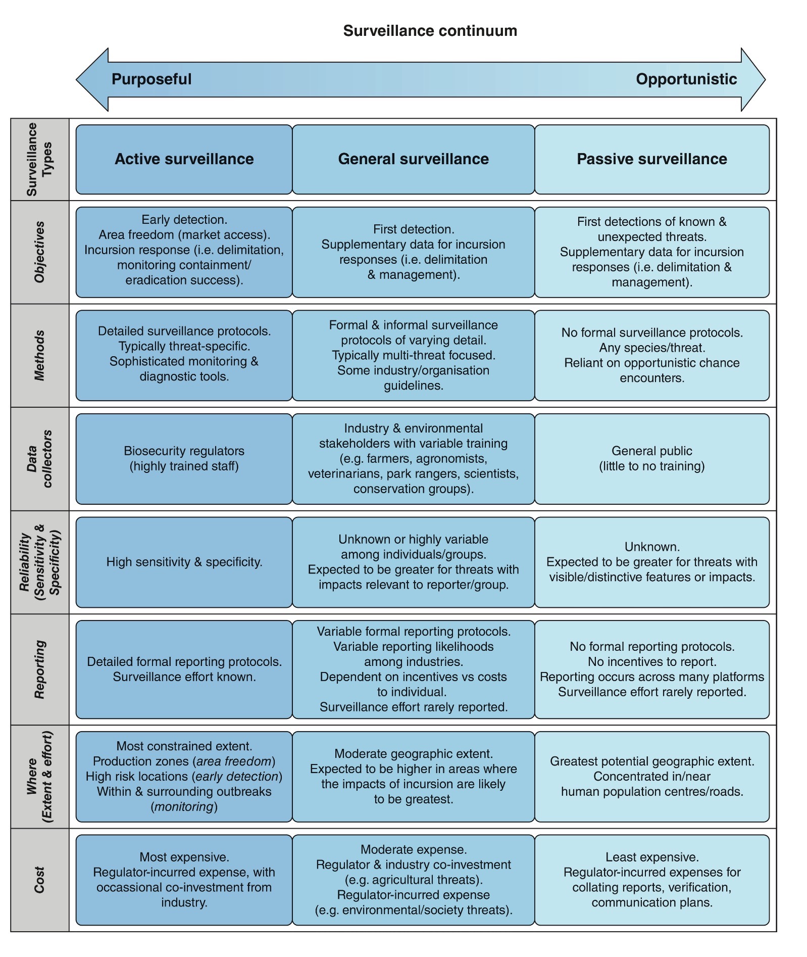 Characteristics of active, general, and passive surveillance (Camac 2024).
The Surveillance Design workflow is intended primarily for active surveillance, where surveillance effort, detection probabilities, and operational costs can be explicitly quantified and optimised. This makes it possible to compare alternative surveillance strategies and allocate resources to maximise the probability of detection within a specified budget or achieve a desired level of confidence at minimum cost.
Existing surveillance activities can also be incorporated into the analysis. For example, estimates of background detection arising from general or passive surveillance—such as public reporting, industry observations, or routine regulatory activities—can be combined with active surveillance to evaluate the overall performance of an integrated surveillance system. In this context, active surveillance is used to complement rather than replace existing detection capability.
When incorporating general or passive surveillance, users should carefully consider how surveillance effort and surveillance unit sensitivity are quantified. Unlike active surveillance, these quantities are often not directly measured and may need to be estimated from expert judgement, historical detection data, reporting rates, or other supporting evidence. These estimates are then used to derive spatially explicit heat maps of the probability of detection, which can be integrated with active surveillance to assess overall system performance.
Representing Surveillance Effort
Within active surveillance, surveillance effort can be represented in different ways depending on how resources are deployed and measured. Broadly, surveillance falls into two categories (Kean et al. 2015):
- Discrete surveillance, where effort is allocated as a countable number of sampling units (e.g. traps, diagnostic tests, inspections, or field surveys).
- Continuous surveillance, where effort is allocated as a continuous quantity (e.g. survey hours, search effort, or area searched).
Biosecurity Commons supports both approaches through its Discrete Sampling and Continuous Surveillance design methods. Selecting the appropriate method ensures that surveillance effort and detection probabilities are modelled consistently with the surveillance program being designed.
Discrete surveillance (Discrete Sampling)
Discrete surveillance is appropriate when surveillance consists of a countable number of sampling units, such as traps, diagnostic tests, plant inspections, animal inspections, or field surveys. The optimisation determines how many sampling units should be allocated to each location to best achieve the chosen surveillance objective.
Detection probability is estimated as a function of the number of samples collected, the sensitivity of each sample, and either the design prevalence (for diseases) or the design population size (for invasive species). This approach is appropriate whenever surveillance effort can be naturally expressed as whole sampling units.
Continuous surveillance (Continuous Surveillance)
Continuous surveillance is appropriate when surveillance effort is more naturally represented as a continuous quantity rather than individual sampling units. Instead of allocating a fixed number of traps or surveys, users allocate an amount of surveillance effort across the landscape.
Biosecurity Commons supports two forms of continuous surveillance:
- Continuous area sampling, where surveillance is allocated as an area searched or monitored (e.g. detector coverage, survey transects, or the effective search area of traps). Detection probability increases with the cumulative area sampled.
- Continuous effort, where surveillance is allocated as an amount of effort (e.g. survey hours, personnel time, or search effort). Detection probability increases as additional surveillance effort is invested.
Continuous surveillance is particularly useful when surveillance effort can be flexibly distributed across space or when the surveillance method cannot be naturally represented as a discrete number of sampling units.
Representing the Surveillance Environment
Biosecurity Commons allows surveillance resources to be allocated across three different types of environments, depending on how the surveillance problem is represented. This flexibility enables the workflow to support surveillance planning across continuous landscapes, discrete locations, or non-spatial management units.
Raster grids
Raster grids are used when surveillance is designed across a continuous landscape. The study region is divided into regularly sized grid cells, with surveillance effort allocated independently to each cell. This approach is well suited to landscape-scale surveillance where risk varies continuously across space, such as allocating surveillance effort across a national establishment risk map or a habitat suitability surface. Raster-based designs typically produce surveillance allocation maps that can be readily visualised and interpreted.
Conforming layers to the region raster
When using a raster to define a region of interest, users can incorporate other raster layers (e.g. for defining occurrence probability). Such rasters may come from other projects or models, and as a consequence, may handle undefined (NA) cells differently, or may have a different distribution of non-NA and NA cells dependent on data inputs. Biosecurity Commons allows users to define how NAs should be handled in two ways:
- Zero undefined values (Default): Any cells with undefined (NA) values that do not correspond to undefined (NA) values in the region layer will be set to zero. This default method is useful when available model layers differ in their spatial distribution of defined (non-NA) and undefined (NA) value cells.
- Nearest define values: Any cells with undefined (NA) values that do not correspond to undefined (NA) values in the region layer will be set to the mean value of the nearest cell(s) with defined values. This method is useful for correcting mismatching borders or coastlines, especially those with differing resolutions.
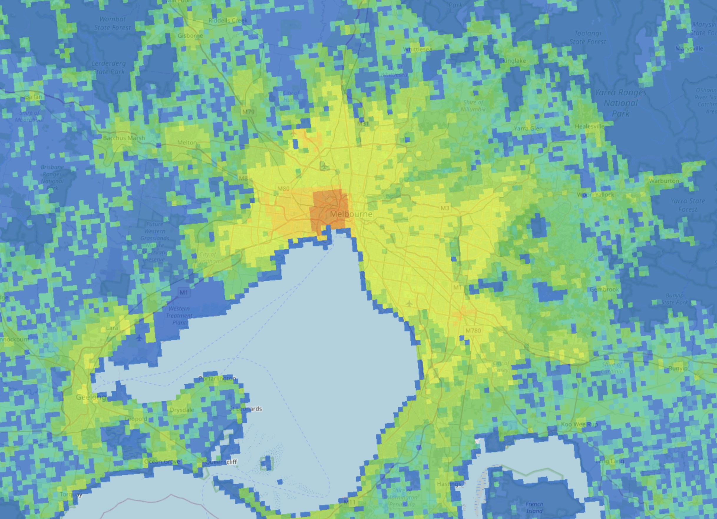
Example establishment probability map (i.e. risk map from Biosecurity Commons).
Spatial locations
Spatial locations are used when surveillance is allocated among a discrete set of known locations defined by geographic coordinates, such as farms, orchards, ports, surveillance sites, or trapping locations. Rather than distributing effort across a continuous surface, the workflow determines how surveillance should be allocated among these individual locations.
Other (aspatial) divisions
Surveillance can also be allocated across non-spatial management units that do not have defined geographic coordinates. These may include categories such as species, production systems, industries, commodities, administrative regions, or other user-defined groupings. This allows the optimisation framework to be applied wherever surveillance resources must be allocated among competing units, even when those units are not spatially explicit.
Occurrence Probability (or Relative Weight)
One of the key inputs to the Surveillance Design workflow is the Occurrence Probability (or Relative Weight) input, which represents the likelihood that the target species occurs within each raster cell, spatial location, or aspatial division. These values are used to prioritise surveillance towards locations where detections are expected to provide the greatest benefit. Although this input is labelled Occurrence Probability, the quantity it represents depends on the surveillance objective. For early detection, it typically represents the probability of initial establishment, whereas for incursion delimitation and response it more commonly represents the probability of current occupancy following spread. Depending on the optimisation objective, this input can be specified either as absolute occurrence probabilities or relative occurrence weights. How these values are estimated depends on the surveillance objective.
Early detection surveillance
For early detection, the Occurrence Probability input typically represents the likelihood of initial establishment. In Biosecurity Commons, these values are most commonly derived from the Risk Mapping workflow, which estimates establishment likelihood by combining information on arrival, abiotic suitability, and biotic suitability. The resulting establishment likelihood map can be supplied directly as the Occurrence Probability input, allowing surveillance to be concentrated where new incursions are most likely to establish. This represents the primary linkage between the Risk Mapping and Surveillance Design workflows.
Incursion delimitation and response
Once an incursion has been detected, the surveillance objective shifts from detecting the first incursion to determining where the pest has spread. In these situations, the Occurrence Probability input is more appropriately informed by the Population Spread Modelling workflow, which predicts the spatial distribution of occupancy or abundance following introduction. These predictions can be supplied directly as the Occurrence Probability input, enabling surveillance to be prioritised towards locations most likely to contain undetected populations. This is particularly useful for outbreak delimitation, containment, and eradication programs. Predicted occupancy through time can also be used to evaluate alternative surveillance strategies for reducing time to detection following an incursion. This represents the primary linkage between the Population Spread Modelling and Surveillance Design workflows.
Absolute probabilities versus relative weights
Occurrence probabilities may also be informed by expert elicitation, previous surveillance programs, historical detections, or other predictive models. Regardless of their source, the Occurrence Probability (or Relative Weight) input can be specified as either absolute probabilities or relative weights, depending on the optimisation objective.
An absolute probability represents the estimated probability that the target species occurs within a particular raster cell, spatial location, or aspatial division. For example, if two locations have occurrence probabilities of 0.02 and 0.10, there is an estimated 2% and 10% chance, respectively, that the species occurs at those locations.
By contrast, a relative weight is a dimensionless quantity that describes the relative distribution of occurrence likelihood across the study region. The magnitude of each value is meaningful only relative to the other locations in the study region and does not represent the actual probability that the species occurs. For example, if one location has a relative weight of 10 and another has a relative weight of 5, the first location is interpreted as being twice as likely to contain the species as the second, but the actual probabilities of occurrence remain unknown. Relative weights therefore identify where the species is more likely to occur, but not how likely it is to occur.
The choice between absolute probabilities and relative weights depends on the optimisation objective:
- Relative weights are appropriate when only the relative spatial distribution of occurrence likelihood is known, or when the objective is simply to prioritise surveillance among locations. They can be used for optimisation objectives such as maximising the expected number of detections or maximising non-monetary benefits, where only the relative ranking of locations influences the optimal surveillance allocation.
- Absolute probabilities are required whenever the optimisation depends on the overall probability of occurrence. This includes estimating system-wide sensitivity (the probability of detecting at least one incursion somewhere within the surveillance system), minimising expected surveillance and management costs, and maximising expected monetary savings, where the expected value of surveillance depends on the actual likelihood that an incursion occurs.
Detection Parameters
The Parameters section defines how an allocation of surveillance effort is converted into a probability of detecting the target species, conditional on it being present. The required parameters depend on whether surveillance is represented as discrete sampling, discrete detection devices, or continuous surveillance.
These detection probabilities are subsequently combined with the Occurrence Probability (or Relative Weight) input to evaluate or optimise the surveillance system.
Discrete sampling
Discrete sampling applies when surveillance involves selecting susceptible units from a population, such as inspecting plants, testing animals, sampling herds, or surveying properties.
The key parameter is sample sensitivity (S): the probability that an individual sample detects the target when the sampled unit is infected or infested.
Detection also depends on the design prevalence (p), which is the minimum proportion of susceptible units assumed to be infected or infested that the surveillance program is designed to detect. A design prevalence of 0.01, for example, means that surveillance is designed to detect the target when 1% of the susceptible population is affected.
When the total population is known
Where the total number of susceptible units is known, Biosecurity Commons calculates the probability of detecting at least one affected unit as:
where
S = sensitivity of each sampled unit
n = number of units sampled
N = total number of susceptible units
p = design prevalence
Here, pN, represents the assumed number of affected units in the population, while n/N, represents the proportion of the population sampled. The equation (Kean et al. 2015) accounts for both the probability that an affected unit is included in the sample and the probability that the surveillance method detects it.
When the total population is unknown
Where the total number of susceptible units is unknown, Biosecurity Commons uses:
where
S = sensitivity of each sampled unit
p = design prevalence
n = number of units sampled
This approximation assumes that no more than approximately 10% of the susceptible population is sampled (Kean et al. 2015). Under that assumption, the probability that any sampled unit is both affected and successfully detected is approximately Sp.
Selecting a design prevalence
Design prevalence is not an estimate of the current prevalence. It is a design threshold: the minimum level of infection or infestation at which the surveillance system should achieve its specified detection performance.
It should be selected by considering:
- the number of susceptible units in the surveillance area;
- the smallest outbreak that must be detected to retain a realistic prospect of containment or eradication;
- the consequences of failing to detect an outbreak at that size; and
- the surveillance effort and cost required to detect increasingly rare outbreaks.
Lower design prevalences imply a requirement to detect smaller outbreaks, but they also require substantially greater surveillance effort. We recommend translating prevalence into an implied number of affected units. For example, a prevalence of 1% in a population of one million host plants corresponds to an outbreak of 10,000 affected plants; practitioners should assess whether an outbreak of that size is operationally tolerable. For many non-disease invasive species, a minimum detectable population size may therefore be more interpretable than prevalence alone.
Discrete detection devices
Prevalence and the total number of susceptible units are not generally required when discrete surveillance represents detection devices such as traps, sensors, cameras, or other devices whose sensitivity is defined directly at the incursion level.
In this context, unit sensitivity is the probability that one deployed device detects the target during the specified surveillance interval, conditional on the target being present in the location (Kean et al. 2015). If devices act independently and have a common sensitivity S, the combined probability of at least one detection from n devices is:
where
S = sensitivity of each surveillance unit (e.g. trap, sensor, or camera)
n = number of surveillance units deployed
The interpretation of S must include the relevant deployment period and detection context. For example, a trap sensitivity may represent the probability of detecting an established local population during one month, rather than the probability of detecting an individual organism during a single encounter.
Continuous surveillance
For continuous surveillance effort (Kean et al. 2015), Biosecurity Commons uses a detection-rate parameter,λ, such that:
where
λ = detection rate (or efficacy) per unit of surveillance effort
E = allocated surveillance effort (e.g. survey hours, search effort, or personnel time)
A larger value of λ means detection probability increases more rapidly as effort increases. Unlike sensitivity, λ is not itself a probability: it is a rate with units that are the inverse of the effort measure, such as per survey hour.
For continuous area sampling, the corresponding formulation is:
where
S = sample sensitivity
A = area sampled (or effectively searched)
D = design density of the target organism (minimum density the surveillance system is designed to detect)
This is the continuous-area analogue of specifying the population level that surveillance is intended to detect.
Estimating sensitivity and detection rates
Sensitivity (S) and λ;can vary with the target species, surveillance method, population density, observer expertise, environmental conditions, deployment duration, and local habitat (Camac 2024). Estimates should therefore match the spatial area and time interval represented in the workflow.
They may be obtained from controlled experiments, field trials, published studies, operational surveillance data, estimates for comparable species or methods, or structured expert elicitation where empirical evidence is unavailable. Because these parameters are often uncertain, alternative designs should be evaluated across a plausible range of sensitivity or λ values.
Surveillance Allocation
The Allocation section determines whether the workflow evaluates an existing surveillance program or identifies an improved surveillance design. Biosecurity Commons supports two allocation modes: Existing Surveillance and Optimised Surveillance. The appropriate choice depends on whether the objective is to assess the performance of a current surveillance system or determine how surveillance resources should be allocated to best achieve a specified management objective.
Existing Surveillance
The Existing Surveillance option evaluates the performance of an existing surveillance network by calculating the detection probability for each location and the resulting system-wide sensitivity. This allows users to determine whether a surveillance program provides sufficient confidence of detecting an incursion, compare alternative surveillance designs, identify gaps in surveillance coverage, or quantify surveillance sensitivity for subsequent Proof of Freedom analyses. No optimisation is performed; the workflow simply evaluates the surveillance allocation supplied by the user.
Optimised Surveillance
The Optimised Surveillance option identifies how surveillance resources should be allocated to best achieve a specified management objective while satisfying user-defined operational constraints. Unlike Existing Surveillance, which evaluates the performance of a user-defined surveillance design, optimisation searches the feasible solution space to identify the surveillance allocation that best satisfies the selected objective.
Selecting an appropriate optimisation objective is critical because different surveillance objectives require different surveillance designs. For example, a surveillance program designed for early detection will often require a different allocation of resources to one designed for incursion delimitation or cost-effective surveillance. The table below summarises the optimisation objective typically recommended for each surveillance objective.
| Surveillance Objective | Recommended Optimisation | Rationale |
| Early Detection (absolute occurrence probabilities) | Maximise system-wide sensitivity | Maximise the probability of detecting at least one incursion |
| Early detection (relative occurrence weights) | Maximise the expected number of detections | Prioritises surveillance towards locations with the highest relative likelihood of occurrence when absolute probabilities are unavailable |
| Incursion delimitation/response monitoring | Maximise the expected number of detections | Maximises the information available to estimate the extent and distribution of an outbreak (i.e. delimitation) or evaluate the effectiveness of response activities. |
| Minimise response costs | Minimise surveillance & management costs | Minimises the combined expected costs of surveillance & response |
| Maximise return on investment | Maximise net monetary savings | Maximises the expected economic return by balancing surveillance costs against avoided damages and response costs |
| Maximise environmental or social outcomes | Maximise non-monetary benefits | Maximise user-defined benefits, such as biodiversity conservation or protection of other high-value assets |
Optimisation objectives
Optimisation objectives can be broken into three broad categories: detection objectives, economic objectives, and benefit-based objectives.
Detection objectives
Question: Where should surveillance be allocated to maximise the likelihood of detecting the target species?
Maximise system-wide sensitivity
Allocates surveillance to maximise the probability of detecting at least one incursion somewhere within the surveillance system.
Maximise the expected number of detections
Allocates surveillance to maximise the expected number of detections across the surveillance region. Unlike system-wide sensitivity, which considers only whether at least one detection occurs, this objective favours surveillance designs that generate multiple detections, thereby providing greater information about the extent and distribution of an incursion.
Economic objectives
Question: How should surveillance resources be allocated to minimise expected costs or maximise economic return?
Minimise surveillance and management costs
Identifies the surveillance allocation that minimises the combined expected cost of surveillance and incursion management. This objective recognises that increasing surveillance investment may reduce future response costs through earlier detection and seeks the allocation that minimises total expected expenditure.
Users must provide estimates of the management cost if detected and management cost if undetected:
Management cost if detected is the expected total cost of responding to and managing an incursion originating at a given location, assuming it is successfully detected by the surveillance system. This excludes the cost of the initial surveillance being optimised but may include delimiting surveillance, diagnostics, treatment or removal, movement controls, eradication or containment activities, and follow-up surveillance.
Management cost if undetected is the expected total cost of responding to and managing an incursion originating at the same location, assuming it is not detected by the surveillance system. This should account for the likely consequences of delayed detection, including additional population growth, spread to other locations, and any resulting changes in the scale, duration or type of management required. Undetected does not necessarily mean the incursion is never discovered, but rather that it is not detected by the surveillance system being optimised.
Important: Both estimates represent the expected total management costs arising from an incursion originating at a particular location, not simply the cost of treating that location or a unit area of infestation. Costs should be estimated over a consistent time horizon and include comparable cost components. Although delayed detection will often increase management costs, this is not always the case, particularly when eradication is abandoned in favour of less intensive management.
These costs can be estimated using historical responses to similar incursions, response plans and budgets, expert elicitation, or modelling of plausible early- and delayed-detection scenarios. Importantly, the detected and undetected estimates should represent comparable scenarios and use the same time horizon and cost components. In most cases, the cost if undetected will be greater because delayed detection allows the incursion to become larger or more widespread before management begins.
Locations where incursions are more likely and where early detection provides a larger reduction in management costs will generally justify greater surveillance investment.
IMPORTANT NOTE: By default, these management costs do not need to include the broader economic, environmental or social damages caused by the threat. However, where these impacts can be expressed in monetary terms, they may be incorporated into both the detected and undetected cost estimates. Doing so changes the interpretation of the analysis from minimising surveillance and response costs to minimising the broader expected economic cost of an incursion. Also note that this method is only available when using probabilities of occurrence. Relative probabilities cannot be used for this method.
Maximise net monetary savings
Allocates surveillance to maximise the expected net economic benefit of surveillance. Net monetary savings are calculated as the avoided damages and avoided response costs resulting from earlier detection, less the cost of undertaking surveillance.
Users provide an estimate of the saving associated with detecting an incursion per location, representing the costs or losses that could be avoided through earlier detection. This may include avoided production or trade losses, environmental damages where these can be monetised, avoided asset losses, or reductions in future management and response costs.
Savings can be estimated by comparing the expected consequences of early detection with those associated with delayed detection.
The expected saving at a location depends on the probability of the threat establishing, the probability that surveillance will detect it, and the monetary saving associated with detection. The optimisation therefore tends to direct greater surveillance effort towards locations where incursions are more likely and where successful detection is expected to generate the greatest savings.
Unlike Minimise Management Costs, which specifically considers differences in the cost of managing detected and undetected incursions, Maximise Savings can incorporate the broader monetary benefits of detection, including avoided economic damages.
IMPORTANT NOTE: This method is also only available when occurrence probabilities are not relative.
Benefit-based objectives
Question: How should surveillance resources be allocated to maximise environmental, social, or other management benefits?
Maximise non-monetary benefits
Allocates surveillance to maximise a user-defined measure of benefit, such as protecting biodiversity, conserving threatened species, reducing environmental impacts, safeguarding culturally significant assets, or protecting other high-value resources.
Unlike Maximise Savings, the benefit does not need to be expressed in monetary terms. Instead, users provide a numerical benefit value for each location representing the relative importance or value of detecting the threat there.
Benefits could represent, for example, the ecological importance of an area, the value of protecting sensitive assets, social or cultural importance, conservation priorities, or a combined decision-support score. Values should be measured on a consistent scale across all locations, with larger values indicating that detection at that location is more valuable.
The optimisation allocates available surveillance resources to maximise the total expected benefit across the surveillance system. Greater surveillance effort will therefore generally be directed towards locations where the threat is more likely to establish, surveillance is more effective, and successful detection has a greater assigned benefit.
Because benefit values do not need to be expressed in monetary terms, this objective is particularly useful where important environmental, social, cultural or strategic consequences cannot reasonably be converted into dollar values.
Operational constraints
Regardless of the optimisation objective, all surveillance designs are obtained subject to user-defined operational constraints. These constraints define the feasible solution space and ensure that recommended surveillance allocations are both analytically optimal and operationally achievable.
Typical constraints include:
- Available surveillance budget or effort — limits the total surveillance resources available for allocation.
- Required system-wide sensitivity — identifies the minimum surveillance effort required to achieve a specified probability of detecting at least one incursion.
- Minimum or maximum surveillance allocations — ensures that locations receive at least a minimum level of surveillance or prevents excessive surveillance effort being allocated to any single location.
- Location-specific surveillance costs — accounts for differences in surveillance costs among locations, allowing resources to be directed towards the most cost-effective opportunities.
- Fixed surveillance allocations — preserves existing surveillance commitments by requiring specified locations to retain predefined surveillance effort while optimising the remaining available resources.
The final surveillance design therefore represents the best achievable allocation given the selected optimisation objective, the operational constraints, and the assumptions specified by the user.
Common Mistakes & Best Practice
Not clearly defining the surveillance objective
The optimal surveillance design depends on the purpose of the surveillance program. For example, early detection aims to maximise the probability of detecting a new incursion as quickly as possible, whereas incursion delimitation seeks to maximise the number of detections to better define the extent and distribution of an outbreak. Likewise, surveillance designed to minimise response costs or maximise return on investment requires different optimisation objectives.
Best practice: Clearly define the surveillance objective before selecting an optimisation objective. The optimisation objective should directly support the management decision that the surveillance program is intended to inform.
Using occurrence estimates that do not reflect the surveillance objective
The Occurrence Probability input should represent the biological process that the surveillance program is intended to detect. Using occurrence estimates that are inconsistent with the surveillance objective can result in surveillance effort being directed towards the wrong locations. For example, establishment likelihood is appropriate for designing early detection surveillance, whereas predicted occupancy following spread is generally more appropriate for incursion delimitation, containment, and eradication.
Best practice: Ensure that the occurrence estimates used reflect the surveillance objective. Within Biosecurity Commons, outputs from the Risk Mapping workflow are generally most appropriate for early detection surveillance, while outputs from the Population Spread Modelling workflow are better suited to surveillance following an incursion.
Including the known incursion or containment zone when optimising delimitation surveillance
The objective of incursion delimitation is to determine the spatial extent of an outbreak, not to confirm the presence of the pest within the known infested area. When the known incursion site, treatment area, or containment zone is included within the optimisation region, the optimiser will naturally allocate surveillance to these locations because they have the highest probability of detection. Although this maximises the expected number of detections, it provides little additional information about the boundary of the outbreak and can reduce surveillance effort in the surrounding areas where the true extent of the incursion remains uncertain.
Best practice: Define the optimisation region so that it excludes the known incursion site, treatment area, or containment zone. Delimitation surveillance should instead focus on the surrounding area where the presence or absence of the pest remains uncertain. In other words, the optimisation should seek to define the uncertain boundary of the outbreak rather than re-survey the known infestation.
Using poorly defined detection parameters
The quality of a surveillance design depends heavily on the estimates of unit sensitivity (Discrete Sampling) or the detection rate (λ) (Continuous Surveillance). These parameters are often uncertain and are sometimes assigned arbitrary values without supporting evidence, which can substantially bias estimates of surveillance performance and the resulting surveillance allocation.
Best practice: Wherever possible, estimate detection parameters from published literature, experimental studies, field trials, or operational surveillance data. If empirical data are unavailable, use a structured expert elicitation process rather than relying on unsupported assumptions or "best guesses". Where uncertainty remains, evaluate surveillance designs across a plausible range of parameter values to assess how sensitive the recommended allocation is to uncertainty.
Selecting an arbitrary design prevalence
Design prevalence represents the minimum prevalence that the surveillance system is designed to detect, not an estimate of the true prevalence. Selecting values such as 1% or 5% without considering what they represent in terms of the number of infected or infested individuals can result in surveillance systems that are either impractical or insufficiently sensitive.
Best practice: Consider the implied number of infected or infested individuals corresponding to the selected design prevalence and determine whether this represents a meaningful management threshold. Where possible, define the smallest outbreak that must be detected to support the surveillance objective, then derive an appropriate design prevalence (or design population size) from that threshold.
Confusing absolute probabilities with relative weights
The Occurrence Probability input can represent either absolute probabilities or relative occurrence weights, depending on the optimisation objective. Treating relative weights as absolute probabilities can produce misleading estimates of system-wide sensitivity and expected surveillance performance.
Best practice: If the overall probability of occurrence cannot be estimated with reasonable confidence, specify the input as relative weights. Absolute probabilities should only be used when they can be meaningfully estimated and are required by the selected optimisation objective.
Assuming surveillance should simply be allocated to the highest-risk locations
Although higher-risk locations generally warrant greater surveillance effort, allocating all surveillance resources to the highest-risk locations is rarely optimal. Effective surveillance design also depends on detection probabilities, surveillance costs, operational constraints, and the chosen optimisation objective.
Best practice: Allow the optimisation framework to balance occurrence probability, detection efficiency, surveillance costs, and operational constraints, rather than allocating surveillance solely according to occurrence likelihood.
Assuming more surveillance always produces a better surveillance design
Increasing surveillance effort generally increases detection probability, but surveillance resources are finite. Beyond a certain point, additional surveillance often produces diminishing improvements in detection while substantially increasing costs.
Best practice: Focus on achieving the greatest improvement in surveillance performance per unit of effort or cost, rather than simply maximising surveillance intensity. The purpose of optimisation is to identify the most efficient allocation of available resources.
Ignoring uncertainty
Occurrence probabilities, detection parameters, surveillance costs, and management benefits are all subject to uncertainty. Optimising surveillance using a single set of parameter values can create a false impression of precision and lead to overconfidence in the recommended surveillance design.
Best practice: Evaluate alternative scenarios by varying key assumptions, particularly occurrence probabilities, detection parameters, design prevalence, and management costs or benefits. Surveillance designs that perform well across a range of plausible assumptions are generally more robust for operational decision-making.
Confusing surveillance allocation with proof of freedom
The Surveillance Design workflow determines where surveillance resources should be allocated to maximise detection or achieve another optimisation objective. It does not determine how much surveillance is required at an individual location, how frequently a location should be resampled, or the confidence that can be placed in zero detections.
Best practice: Use the Surveillance Design workflow to optimise the spatial allocation of surveillance resources across locations. If the objective is to estimate confidence that a pest is absent following zero detections or determine the surveillance effort required to demonstrate freedom, use the Proof of Freedom workflow instead. Existing surveillance designs can be exported directly from Surveillance Design to Proof of Freedom for this purpose.
Confusing risk maps with surveillance designs
Risk maps identify where an invasive species is most likely to occur, but they do not identify the optimal surveillance allocation. Effective surveillance design depends not only on occurrence probability, but also on detection probabilities, surveillance costs, operational constraints, and the surveillance objective. Consequently, allocating surveillance directly according to a risk map is unlikely to produce the most effective surveillance design.
Best practice: Use occurrence models, such as establishment likelihood or predicted occupancy maps, to inform the Occurrence Probability input, then allow the optimisation framework to determine how surveillance resources should be allocated to best achieve the selected surveillance objective.
Want to use our R package?
Biosecurity Commons is powered by a number of specially built R packages. If you would like to use our optimal surveillance design methods in R please visit our bsdesign GitHub page
References
- Anderson, D. P., Gormley, A. M., Ramsey, D. S. L., Nugent, G., Martin, P. A. J., Bosson, M.,Livingstone, P., & Byrom, A. E. (2017). Bio-economic optimisation of surveillance to confirm broadscale eradications of invasive pests and diseases.Biological Invasions, 19(10), 2869–2884.
- Camac, J. S. (2024). Detect: Designing post-border surveillance schemes. In Hester et al. (Eds.), Biosecurity: A Systems Perspective. Taylor & Francis.
- Hauser, C. E., & McCarthy, M. A. (2009). Streamlining ’search and destroy’: cost-effective surveillance for invasive species management. Ecology Letters, 12(7), 683–692.
- Kean, J. M., Burnip, G. M. & Pathan, A. (2015). Detection survey design for decision making during biosecurity incursions. In F. Jarrad, S. Low-Choy & K. Mengersen (eds.), Biosecurity surveillance: Quantitative approaches (pp. 238– 250). Wallingford, UK: CABI.
- McCarthy, M. A., Thompson, C. J., Hauser, C., Burgman, M. A., Possingham, H. P., Moir, M. L.,Tiensin, T., & Gilbert, M. (2010). Resource allocation for efficient environmental management. Ecology Letters, 13(10), 1280–1289.
- Moore, A. L., McCarthy, M. A., & Lecomte, N. (2016). Optimizing ecological survey effort overspace and time. Methods in Ecology and Evolution, 7(8), 891–899.
Was this article helpful?
That’s Great!
Thank you for your feedback
Sorry! We couldn't be helpful
Thank you for your feedback
Feedback sent
We appreciate your effort and will try to fix the article