Proof of freedom - how many rounds of surveillance?

This article is focused on providing a more in-depth understanding of the Proof of Freedom workflow. If you are interested in a step-by-step guide on how to use the Biosecurity Commons interface for Proof of Freedom please see our Proof of Freedom Quick Start Guide.

Overview

Preventing the establishment of exotic pests, weeds, and diseases relies on a combination of pre-border measures, border interventions, and post-border surveillance. While pre-border activities reduce the likelihood of introduction, no biosecurity system can eliminate risk entirely. Consequently, surveillance remains a fundamental component of biosecurity systems, enabling authorities to detect incursions early, delimit their extent, demonstrate successful eradication, and provide evidence that an area remains free from a target organism (Camac 2024).

The Surveillance Design workflow in Biosecurity Commons helps users determine where surveillance should be conducted and how much surveillance effort is required to achieve a desired probability of detection. In contrast, the Proof of Freedom (PoF) workflow addresses the complementary question of how many rounds of surveillance, or how much time, are required before there is sufficient statistical evidence that a target organism is absent if it has not been detected.

Proof of Freedom methods combine information about the sensitivity of a surveillance system (i.e. the likelihood it detects the threat of interest) with the outcomes of repeated surveillance to quantify confidence that an area is free from a target organism. Confidence increases as additional surveillance is conducted without detection, although the rate at which confidence accumulates depends on factors such as surveillance sensitivity, the number of repeat surveys, and assumptions regarding the probability of reintroduction and population persistence.

Demonstrating area freedom is a fundamental component of biosecurity decision-making. Statistical evidence of freedom underpins declarations of pest- or disease-free status, supports claims of successful eradication, informs decisions to transition from emergency response to routine surveillance, and provides the evidence required to maintain or restore domestic and international market access (Camac 2024). By quantifying confidence that a target organism is absent, proof of freedom provides an objective and transparent basis for decisions that have important regulatory, economic, and environmental consequences. The Biosecurity Commons Proof of Freedom workflow enables users to estimate confidence in area freedom from surveillance data using either historical detection records or estimates of surveillance system sensitivity. The workflow can be used to:

• quantify how confidence in area freedom increases following repeated surveillance with no detections;
• determine the number of surveillance rounds or the period of surveillance required to achieve a specified confidence level (e.g. 95% confidence of freedom);
• assess how changes in surveillance sensitivity influence the time required to demonstrate freedom; and
• account for uncertainty in surveillance sensitivity, historical surveillance performance, and the risk of pathogen or pest reintroduction or persistence between surveillance events.

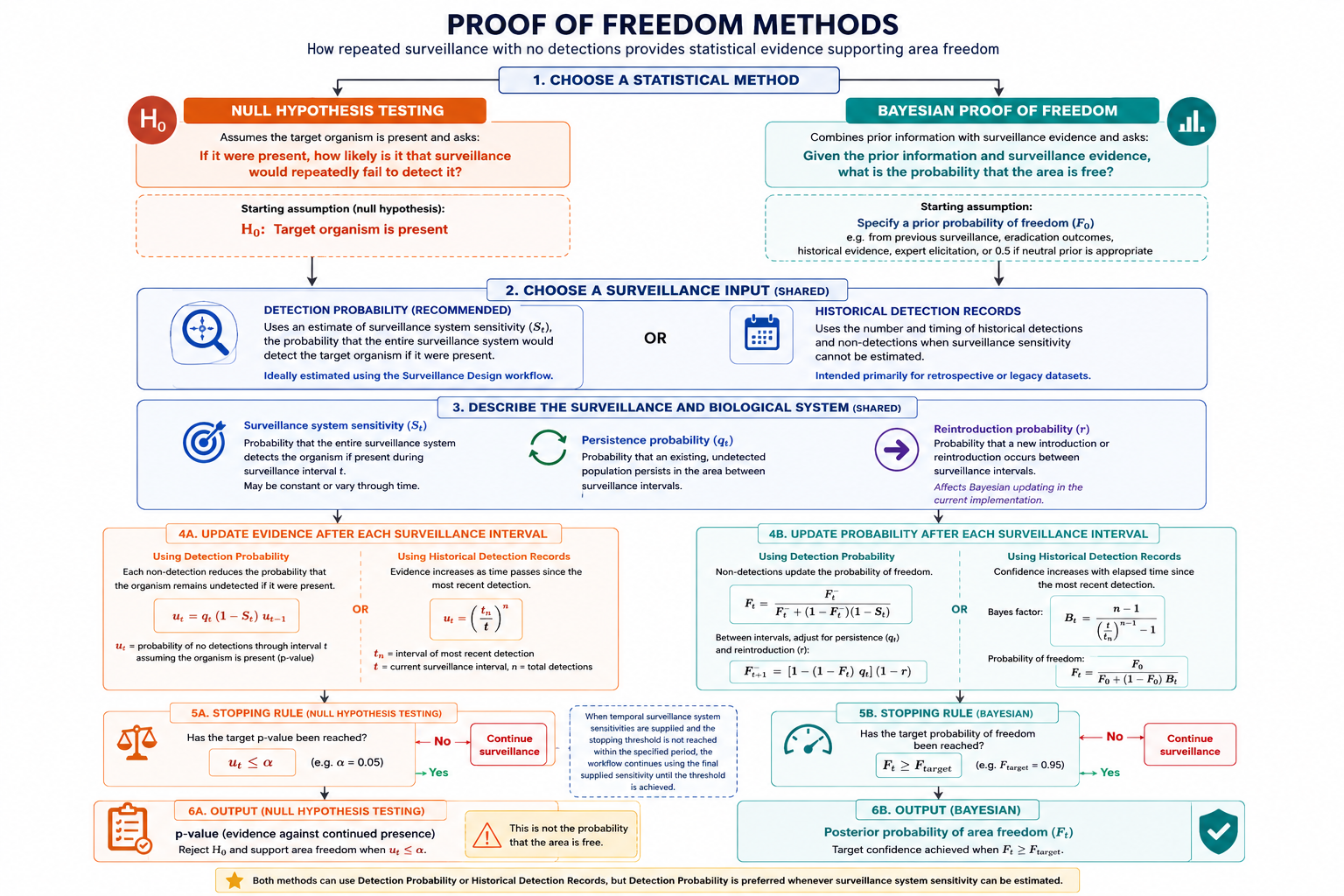
Shematic of Proof of Freedom workflow. 

Choosing a Proof of Freedom Method

Biosecurity Commons provides two complementary statistical approaches for demonstrating area freedom:

• Hypothesis Test Proof of Freedom – evaluates the hypothesis that the target organism remains present despite not being detected. As surveillance accumulates without detection, the probability that the organism remains present decreases. When this probability falls below a specified threshold (e.g. 0.05), the hypothesis of presence can be rejected, providing statistical support for a claim of area freedom (e.g. 95% confidence). This method allows users to account for likelihood of threat persistence between survey rounds. However, it does not account for likelihoods of re-introduction between events.
• Bayesian Proof of Freedom – applies Bayes' theorem to iteratively update the probability that an area is free from the target organism. This approach combines surveillance outcomes with a prior belief about freedom and naturally accommodates information from previous surveillance, expert judgement, and estimates of reintroduction and persistence risk.

Both methods use surveillance information collected over one or more surveillance rounds to quantify evidence supporting area freedom. As additional surveillance is conducted without detecting the target organism, evidence supporting freedom increases. The primary difference between the methods lies in how they interpret that evidence.

The Hypothesis Testing approach evaluates whether there is sufficient evidence to reject the hypothesis that the target organism remains present. By contrast, the Bayesian approach estimates the probability that an area is free by combining surveillance evidence with existing knowledge or beliefs about the likelihood that the target organism is absent.

Neither approach is universally superior. The most appropriate method depends on the management context, the information available before surveillance begins, and whether meaningful prior information exists.

Hypothesis Testing Proof of Freedom

The hypothesis testing approach begins by assuming that the target organism is present within the surveillance area (Rout 2017; Camac 2024). This assumption forms the null hypothesis.

Each round of surveillance that fails to detect the target organism reduces the probability that the organism could still be present while remaining undetected. This probability is expressed as a p-value, representing the strength of evidence against the null hypothesis. When the p-value falls below a user-defined significance threshold (typically 0.05), the null hypothesis that the organism remains present can be rejected, providing statistical support for a claim of area freedom (e.g. 95% confidence, accepting a 5% probability of incorrectly rejecting the null hypothesis).

Importantly, this method does not estimate the probability that an area is free. Rather, it evaluates whether the available surveillance evidence is sufficiently inconsistent with the assumption that the organism is still present.

In other words, it asks:

If the target organism were still present, how likely is it that we would have observed no detections?

If that probability is sufficiently small, continued presence is considered unlikely and area freedom is supported.

Advantages

• Does not require specification of a prior probability of freedom.
• Provides an objective and transparent assessment based solely on surveillance outcomes.
• Familiar to many regulators and scientists through classical statistical hypothesis testing.
• Straightforward to interpret when surveillance begins with little or no prior information.

Limitations

• Does not incorporate previous surveillance or other evidence collected before the current analysis.
• Every analysis effectively begins from the same assumption that the organism may be present.
• Does not directly estimate the probability that an area is free. Instead, absence is inferred from the probability that the organism would have escaped detection if it were present.

Recommended applications

The hypothesis testing approach is generally most appropriate when:

• little or no prior information exists regarding the status of the target organism;
• regulatory frameworks require classical hypothesis testing; or
• an objective assessment without subjective prior assumptions is preferred.

Bayesian Proof of Freedom

The Bayesian approach treats proof of freedom as an iterative process of updating evidence through time.

Rather than assuming the organism is present, Bayesian inference begins with a prior probability of freedom, representing the confidence that the target organism is absent before surveillance begins (Examples: Magarey et al. 2019; Anderson et al 2022). This prior is updated following each surveillance round using Bayes' theorem.

Unlike the hypothesis testing approach, Bayesian inference allows previous surveillance, expert judgement, eradication outcomes, historical evidence, or other sources of information to contribute formally to the analysis.

When a neutral prior of 0.5 is specified, the Bayesian approach assumes that the target organism is equally likely to be present or absent before surveillance begins. Under this assumption, Bayesian and hypothesis testing approaches often produce very similar trajectories of increasing evidence following repeated surveillance with no detections. However, the two methods remain conceptually distinct. The hypothesis testing approach evaluates evidence against continued presence, whereas the Bayesian approach estimates the probability that an area is free given the available evidence.

As more informative prior knowledge becomes available, the Bayesian approach becomes increasingly advantageous because it allows surveillance to build upon previous evidence rather than treating every analysis independently.

Advantages

• Explicitly incorporates prior information and previous surveillance.
• Naturally updates confidence as surveillance progresses.
• Produces a direct estimate of the probability of area freedom.
• Well suited to long-term surveillance programs.
• Provides a flexible framework for incorporating expert judgement and uncertainty.

Limitations

• Requires specification of a prior probability of freedom.
• Results can be influenced by the selected prior, particularly during the early stages of surveillance.
• Prior probabilities should be scientifically justified wherever possible.

Recommended applications

The Bayesian approach is generally preferred when:

• previous surveillance has already provided evidence of area freedom;
• the target organism has previously been detected and an eradication program has been undertaken;
• historical surveillance information exists;
• expert knowledge regarding the likelihood of freedom is available; or
• surveillance is conducted repeatedly over many years.

Choosing Between Methods

For many surveillance programs the two approaches produce very similar conclusions, particularly after many rounds of surveillance. Differences are generally greatest during the early stages of surveillance because only the Bayesian method incorporates prior information.

The Bayesian method becomes increasingly advantageous whenever meaningful prior information exists. For example, following an eradication program there may already be substantial evidence that the target organism has been eliminated. Similarly, long-term surveillance programs often accumulate historical evidence that should contribute to current assessments. In these situations, incorporating prior information provides a more realistic estimate of confidence in area freedom than treating every surveillance program as though it were beginning from scratch.

Conversely, when little or no prior information is available, the hypothesis testing approach provides a simple and objective framework that depends solely on the observed surveillance outcomes.

When no defensible prior probability exists, specifying a neutral prior of 0.5 often produces a trajectory of increasing confidence that closely resembles the hypothesis testing approach while retaining the advantages of Bayesian updating.

Detection Input data

Both the Hypothesis Testing and Bayesian workflow supports two alternative sources of surveillance information:

• Detection Probability (recommended)
• Historical Detection Records

Although both inputs ultimately estimate the probability that the target organism would remain undetected if present, they differ substantially in the information they require and the assumptions they make.

Detection Probability

The Detection Probability approach uses an explicit estimate of the surveillance system sensitivity (also referred to as the probability of detection given presence) for each surveillance round.

This is the preferred approach because it directly quantifies the ability of the surveillance system to detect the target organism if it were present. Detection probability may be estimated using the Biosecurity Commons Surveillance Design workflow or derived independently through surveillance evaluation, simulation modelling, expert elicitation, or previous surveillance studies.

By explicitly modelling surveillance sensitivity, this approach naturally accounts for differences in surveillance effort between surveillance rounds. Increasing survey effort, deploying more traps, inspecting more hosts, improving diagnostic tests, or allocating surveillance to higher-risk locations all increase surveillance sensitivity and therefore reduce the probability that an existing population remains undetected.

Historical Detection Records

The Historical Detection Record approach is intended primarily for situations where surveillance sensitivity cannot be estimated.

Rather than explicitly modelling surveillance effectiveness, this approach estimates evidence supporting area freedom using only the timing and sequence of historical detections and non-detections. Confidence in area freedom increases as additional surveillance periods occur without further detections following the most recent detection.

Because surveillance sensitivity is unknown, this method implicitly assumes that surveillance effort and surveillance effectiveness have remained broadly comparable through time. Consequently, it should be regarded as an empirical approximation rather than a fully mechanistic proof of freedom analysis.

This approach is particularly useful for historical surveillance datasets where only detection histories have been retained and no information exists regarding surveillance effort, trap density, inspection intensity, or diagnostic performance (Solow 1993; Rout 2017).

Which input should I choose?

Whenever possible, Biosecurity Commons recommends using Detection Probability.

Detection Probability explicitly quantifies the effectiveness of the surveillance system and therefore provides a more realistic and scientifically defensible estimate of the probability that an existing population would have escaped detection.

Historical Detection Records should generally be reserved for retrospective analyses or legacy surveillance programs where surveillance sensitivity cannot be estimated.

Specifying the Surveillance System

Regardless of the statistical method selected, the Proof of Freedom workflow requires users to describe the surveillance system and the biological processes influencing the persistence of the target organism. These parameters determine how much evidence is gained from each round of surveillance and therefore how quickly confidence in area freedom accumulates over time.

Careful consideration should be given to each parameter, as they directly influence the resulting estimates of area freedom. Wherever possible, parameter values should be derived from surveillance design analyses, published studies, surveillance evaluations, or expert elicitation rather than arbitrary assumptions.

Surveillance System Sensitivity

Surveillance system sensitivity (also referred to as system sensitivity) represents the probability that the entire surveillance system would detect the target organism during a surveillance round if it were present within the surveillance area.

Surveillance system sensitivity is the primary link between the Surveillance Design and Proof of Freedom workflows. The Surveillance Design workflow estimates the probability that a surveillance system would detect the target organism if it were present, whereas the Proof of Freedom workflow uses this probability to quantify how confidence in area freedom accumulates through repeated surveillance. Consequently, surveillance system sensitivity is arguably the most important parameter within the Proof of Freedom workflow.

Surveillance system sensitivity should not be confused with surveillance unit sensitivity, which describes the probability that an individual surveillance unit (e.g. trap, property, host, or sample) detects the target organism if it is present. Instead, surveillance system sensitivity combines surveillance unit sensitivity with the overall surveillance design, including the number of surveillance units, their spatial distribution, design prevalence, and surveillance effort, to estimate the probability that the surveillance system as a whole would detect the target organism if it were present.

Whenever possible, surveillance system sensitivity should be estimated using the Biosecurity Commons Surveillance Design workflow, which explicitly accounts for surveillance unit sensitivity, surveillance effort, design prevalence, and the spatial allocation of surveillance resources. Alternatively, surveillance system sensitivity may be estimated from surveillance evaluations, simulation modelling, expert elicitation, published studies, or other quantitative assessments of surveillance performance.

Constant versus Temporal Surveillance System Sensitivity

For analyses using the Detection Probability input, Biosecurity Commons supports both:

• Constant surveillance system sensitivity, where surveillance performance is assumed to remain unchanged throughout the analysis; and
• Temporal surveillance system sensitivity, where surveillance performance varies between surveillance rounds.

The temporal option recognises that surveillance systems often change through time. For example, surveillance intensity may increase during an eradication response before gradually declining during post-eradication monitoring. Similarly, surveillance effort may vary between years because of changes in available resources, staffing, surveillance priorities, or surveillance design.

When temporal surveillance system sensitivities are supplied, the workflow automatically updates confidence using the surveillance system sensitivity associated with each surveillance interval. This enables users to evaluate how changes in surveillance effort influence the accumulation of evidence supporting area freedom over time.

Best practice

Whenever possible, estimate surveillance system sensitivity using the Surveillance Design workflow rather than relying solely on expert judgement. This provides a transparent, reproducible, and defensible estimate of surveillance performance that is directly linked to surveillance effort and surveillance design.

Persistence Probability

The Persistence Probability represents the probability that the target organism remains present between successive surveillance rounds if it has not been detected.

By default, this parameter is set to 1.0, implying that an undetected population is assumed to persist indefinitely until detected. This represents a conservative, worst-case assumption because confidence in area freedom can only increase through successful surveillance rather than natural population decline or extinction.

However, some organisms may have a substantial probability of failing to persist between surveillance rounds. For example, transient incursions, unsuccessful establishment attempts, or organisms that cannot survive without suitable hosts may naturally disappear over time. In these situations, specifying a persistence probability less than one allows the workflow to account for the possibility that an undetected population may no longer exist.

Reducing the persistence probability generally results in confidence accumulating more rapidly because the probability of continued undetected presence decreases between surveillance rounds.

Best practice

Unless there is strong biological or epidemiological evidence supporting lower persistence, the default value of 1.0 is recommended. This provides a conservative estimate of area freedom by assuming that an undetected population will persist until detected.

Reintroduction Probability

The Reintroduction Probability represents the probability that the target organism is introduced into the surveillance area between successive surveillance rounds after freedom has been established.

Unlike persistence, which describes the fate of an existing undetected population, reintroduction represents the possibility of a new incursion occurring during the surveillance period.

Where ongoing introduction pathways remain active, confidence in area freedom may decrease between surveillance rounds because a previously free area may become reinfested. Reintroduction is therefore particularly relevant for long-term surveillance programs where the risk of new introductions cannot reasonably be assumed to be negligible.

Although reintroduction probability is often assumed to be zero or very small over relatively short surveillance periods, it may become increasingly important for organisms associated with continual pathways of introduction, such as international trade, natural dispersal from neighbouring regions, or repeated human-mediated movement.

Best practice

For most post-response Proof of Freedom analyses, reintroduction probability will often be assumed to be zero or negligible. However, where continuing introduction pathways are known to exist, users should consider incorporating an appropriate estimate based on pathway risk assessments, surveillance intelligence, or expert judgement.

Stopping Conditions

The Proof of Freedom workflow estimates evidence supporting area freedom iteratively over successive surveillance rounds. Users must therefore specify the condition under which the iterative calculations should terminate.

Stopping conditions determine whether the workflow performs a predefined number of surveillance iterations or continues until a specified level of evidence supporting area freedom has been achieved.

Depending on the selected statistical method, Biosecurity Commons supports the following stopping conditions:

• Number of Iterations
• Target Confidence (Bayesian only)
• Target p-value (Hypothesis Testing only)

Number of Iterations

This option instructs the workflow to perform a fixed number of surveillance iterations.

Each iteration typically represents a surveillance round or time interval (e.g. years, months, survey campaigns, or trapping seasons), depending on the temporal unit selected when configuring the project.

This option is most appropriate when users wish to evaluate how confidence in area freedom changes throughout a predefined surveillance program rather than determine the surveillance duration required to achieve a specified level of confidence.

Target Confidence (Bayesian)

For Bayesian analyses, users may instead specify a target probability of freedom (for example, 95%).

Rather than performing a fixed number of surveillance rounds, the workflow continues iterating until the estimated posterior probability of area freedom reaches or exceeds the specified confidence threshold.

This stopping condition directly answers the management question:

How many surveillance rounds, or how much time, are required before the desired confidence in area freedom has been achieved?

This option is particularly useful when planning surveillance programs or determining the duration of post-eradication surveillance.

Target p-value (Hypothesis Testing)

For Hypothesis Testing analyses, users specify the significance threshold used to reject the null hypothesis that the target organism remains present.

The workflow continues iterating until the calculated p-value falls below the specified threshold (typically 0.05).

This stopping condition answers the complementary management question:

How many surveillance rounds, or how much time, are required before there is sufficient statistical evidence to reject continued presence?

Temporal Surveillance Beyond the Specified Time Period

When temporal surveillance system sensitivities are provided, the workflow initially uses the surveillance system sensitivity associated with each corresponding surveillance interval.

However, the specified stopping condition may not always be achieved within the period covered by the supplied temporal surveillance data.

Rather than terminating the analysis prematurely, Biosecurity Commons assumes that surveillance continues beyond the final specified surveillance interval using the last available surveillance system sensitivity. Subsequent surveillance rounds therefore continue using this final surveillance system sensitivity until the specified stopping condition is reached.

This behaviour reflects the practical assumption that future surveillance is expected to continue with approximately the same surveillance effectiveness as the most recently specified surveillance program unless alternative information is available.

Example

Suppose annual surveillance system sensitivities have been estimated for the first five years following an eradication response:

If the specified stopping condition has not been achieved after Year 5, the workflow automatically assumes that surveillance continues using a surveillance system sensitivity of 0.40 for Years 6, 7, 8 and beyond until the required confidence (Bayesian) or target p-value (Hypothesis Testing) is reached.

This enables users to estimate the total surveillance duration required without explicitly specifying surveillance system sensitivities for an arbitrary number of future surveillance rounds.

Common Mistakes and Best Practices

Confusing proof of freedom with proof of absence

Proof of Freedom does not demonstrate that a target organism is absent with absolute certainty. Rather, it quantifies the statistical evidence supporting area freedom given the surveillance that has been undertaken and the assumptions specified by the user.

Even high confidence values (e.g. 95% or 99%) represent a probability of freedom rather than certainty. Residual uncertainty always remains because no surveillance system is perfectly sensitive.

Best practice: Interpret outputs as the statistical confidence that an area is free given the surveillance evidence and model assumptions, rather than as definitive proof that the target organism is absent.

Overestimating surveillance system sensitivity

Confidence in area freedom accumulates directly as a function of surveillance system sensitivity. If surveillance system sensitivity is overestimated, confidence in area freedom will also be overestimated.

This commonly occurs when surveillance sensitivity is based on optimistic assumptions regarding detection probabilities, survey coverage, diagnostic performance, or observer effectiveness.

Best practice: Estimate surveillance system sensitivity using quantitative surveillance design methods wherever possible. If expert judgement is required, use conservative estimates and document the assumptions used.

Confusing surveillance unit sensitivity with surveillance system sensitivity

A common mistake is to use the probability of detecting the target organism in a single surveillance unit (e.g. one trap, one property, one sample, or one inspection) as the surveillance system sensitivity.

Surveillance system sensitivity represents the probability that the entire surveillance program would detect the target organism if it were present and therefore depends on both surveillance unit sensitivity and surveillance design.

Best practice: Estimate surveillance system sensitivity using the Surveillance Design workflow or another quantitative surveillance design method rather than directly entering surveillance unit sensitivities.

Using surveillance intervals that are not biologically independent

Successive surveillance intervals should represent biologically meaningful opportunities for detecting the target organism. Conducting repeated surveys too frequently may violate the assumption that each surveillance interval provides independent evidence supporting area freedom.

For example, repeating surveys over short time periods when the target organism is inactive, undetectable, or unlikely to have changed in abundance provides relatively little additional information compared with surveys conducted after sufficient time has elapsed.

Similarly, multiple inspections of the same surveillance units over a short period may not provide independent evidence if detectability has not materially changed.

Best practice: Choose surveillance intervals that reflect the biology of the target organism, including its life cycle, seasonal activity, dispersal, detectability, and expected rate of population change. Each surveillance interval should represent a meaningful opportunity for new evidence to accumulate.

Ignoring changes in surveillance effort through time

Surveillance effort often changes between surveillance intervals because of changing budgets, staffing, surveillance priorities, or operational constraints.

Assuming constant surveillance system sensitivity when surveillance effort has changed may either overestimate or underestimate confidence in area freedom.

Best practice: Where surveillance effort varies through time, provide temporal surveillance system sensitivities so that confidence is updated using the appropriate surveillance performance for each surveillance interval.

Assuming persistence when the organism cannot persist (or vice versa)

The persistence probability should reflect the biology of the target organism.

Some organisms readily persist between surveillance intervals, whereas others may naturally fail to establish or survive without suitable environmental conditions or hosts.

Assuming persistence is certain when it is not may underestimate confidence in area freedom, whereas unrealistically low persistence probabilities may produce overconfident results.

Best practice: Base persistence probabilities on biological knowledge of the target organism and use the default value of 1.0 unless there is clear evidence supporting lower persistence.

Ignoring the possibility of reintroduction

Proof of Freedom assumes that confidence accumulates following repeated surveillance. However, confidence may decline if the surveillance area remains exposed to continuing pathways of introduction.

Ignoring reintroduction may therefore overestimate confidence, particularly for long-term surveillance programs or regions exposed to continual invasion pressure.

Best practice: Consider whether ongoing pathways of introduction exist and include a reintroduction probability where appropriate, particularly for long-term surveillance programs.

Using historical detection records when surveillance sensitivity can be estimated

The Historical Detection Record approach provides a practical solution when surveillance system sensitivity cannot be estimated. However, it does not explicitly account for surveillance effort or surveillance effectiveness.

Where surveillance sensitivity can be estimated, analyses based on Detection Probability provide a more realistic and statistically defensible estimate of confidence in area freedom.

Best practice: Use the Detection Probability input whenever surveillance system sensitivity can be estimated. Reserve the Historical Detection Record approach primarily for retrospective analyses and legacy surveillance datasets.

Using an unrealistic prior probability (Bayesian method)

The Bayesian approach allows previous information to contribute to the analysis through the prior probability of freedom.

Selecting an unrealistically high prior may produce overconfident estimates of area freedom, particularly during the early stages of surveillance.

Best practice: Where little prior information exists, use a neutral prior (0.5). Where previous surveillance, eradication programs, or expert knowledge exist, ensure that the selected prior is scientifically justified and clearly documented.

Treating model outputs as independent of their assumptions

Proof of Freedom analyses are only as reliable as the assumptions used to parameterise the surveillance system.

Surveillance system sensitivity, persistence probability, reintroduction probability, surveillance interval, and prior probability (Bayesian method) all directly influence the resulting estimates of confidence.

Best practice: Clearly document all assumptions, explore alternative parameter values using sensitivity analyses where appropriate, and interpret results within the context of the specified assumptions rather than as universally applicable estimates of area freedom.

Mathematical formulation

Null Hypothesis Testing

The hypothesis testing approach assumes that the target organism is present and evaluates the probability of obtaining the observed surveillance results under this assumption.

The null hypothesis is:

Detection Probability

When surveillance system sensitivity is provided, the workflow calculates the probability that the target organism would remain undetected if it were present.

Initial condition

For the first surveillance interval:

Recursive update

For each subsequent surveillance interval:

where

u_t = probability that the target organism remains undetected through surveillance interval t, assuming it is present (the reported p-value)
u_t−1 = probability that the target organism remained undetected through the previous surveillance interval
S_t = surveillance system sensitivity during surveillance interval t
q_t = probability that the target organism persists during the relevant surveillance interval

If persistence is assumed to be certain, such that q_t = 1, the recursive calculation simplifies to:

Decision threshold

Area freedom is statistically supported when:

where

α = selected significance threshold, typically 0.05

Importantly, u_t represents the probability of obtaining no detections if the organism is present. It is not the probability that the organism remains present after observing no detections.

Historical Detection Records

When historical detection records are supplied, the workflow does not use an explicitly estimated surveillance system sensitivity. Instead, it estimates the probability of undetected presence from the number of historical detections and the elapsed time since the most recent detection.

Initial condition

The evidence value remains equal to 1 up to and including the surveillance interval containing the most recent detection:

Historical detection update

For surveillance intervals following the most recent detection:

where

u_t = estimated probability of undetected presence at surveillance interval t
n = total number of historical detections
t_n = surveillance interval corresponding to the most recent detection
t = current surveillance interval

As the elapsed time since the most recent detection increases, u_t decreases. Area freedom is supported when the resulting value falls below the selected significance threshold.

Bayesian Proof of Freedom

The Bayesian approach estimates the probability that an area is free by combining a prior probability of freedom with surveillance evidence. The probability is updated after each surveillance interval using Bayes' theorem.

Detection Probability

When surveillance system sensitivity is provided, the workflow updates the probability of freedom following each surveillance interval in which the target organism is not detected.

Initial condition

The analysis begins with a user-specified prior probability of freedom:

where

F₀ = prior probability that the surveillance area is free before the first surveillance interval
F₁⁻ = probability of freedom immediately before the first surveillance interval

Surveillance update

Following surveillance interval t with no detections, the posterior probability of freedom is:

where

F_t⁻ = probability of freedom immediately before surveillance interval t
F_t = posterior probability of freedom following surveillance interval t
S_t = surveillance system sensitivity during surveillance interval t

Between-interval update

Before the next surveillance interval, the posterior probability is adjusted to account for persistence and the possibility of introduction or reintroduction:

where

F_t+1⁻ = probability of freedom immediately before the next surveillance interval
q_t = probability that the target organism persists between surveillance intervals if it is present
r = probability of introduction or reintroduction between surveillance intervals

If persistence is certain and introduction or reintroduction is assumed not to occur, such that q_t = 1 and r = 0, the posterior probability from one surveillance interval becomes the prior probability for the next:

Stopping threshold

When a target confidence is selected, the analysis stops when:

where

F_target = selected target probability of freedom, such as 0.95

Historical Detection Records

When historical detection records are supplied, the Bayesian workflow estimates confidence in area freedom from the number of detections and the elapsed time since the most recent detection rather than from an explicitly estimated surveillance system sensitivity.

Initial condition

The estimated probability of freedom remains equal to zero up to and including the surveillance interval containing the most recent detection:

Bayes factor

For surveillance intervals following the most recent detection, the Bayes factor is calculated as:

Probability-of-freedom update

The corresponding probability of freedom is:

where

B_t = Bayes factor at surveillance interval t
F₀ = prior probability of freedom
F_t = estimated probability of freedom at surveillance interval t
n = total number of historical detections
t_n = surveillance interval corresponding to the most recent detection
t = current surveillance interval

As the elapsed time since the most recent detection increases, the Bayes factor decreases and the estimated probability of freedom increases.

Important: the historical-record Bayesian calculation requires at least two historical detections because the equation contains n − 1 in both the numerator and exponent. Where only one detection is available, the calculation is not well defined and the Detection Probability approach should be used instead.

Want to use our R package?

Biosecurity Commons is powered by a number of specially built R packages. If you would like to use our optimal surveillance design & proof of freedom methods in R please visit our bsdesign GitHub page

Additional reading

• Anderson, D. P., Gormley, A. M., Ramsey, D. S. L., Nugent, G., Martin, P. A. J., Bosson, M.,Livingstone, P., & Byrom, A. E. (2017). Bio-economic optimisation of surveillance to confirm broadscale eradications of invasive pests and diseases. Biological Invasions, 19(10), 2869–2884.
• Anderson, D. P., Pepper, M. A., Travers, S., Michaels, T. A., Sullivan, K., & Ramsey, D. S. L. (2022). Confirming the broadscale eradication success of nutria (Myocastor coypus) from the Delmarva Peninsula, USA.

  Biological Invasions, 24,3509-3521

• Barclay, H. J., & Hargrove, J. W. (2005). Probability models to facilitate a declaration of pest-free status, with special reference to tsetse (Diptera: Glossinidae). Bulletin Of Entomological Research

  (London), 95(1), 1–12.

• Camac, J. S. (2024). Detect: Designing post-border surveillance schemes. In Hester et al. (Eds.), Biosecurity: A Systems Perspective. Taylor & Francis.
• Magarey, R. C., Reynolds, M., Dominiak, B. C., Sergeant, E., Agnew, J., Ward, A., & Thompson, N. (2019). Review of sugarcane Fiji leaf gall disease in Australia and the declaration of pest freedom in Central Queensland. Crop Protection, 121, 113–120.
• Regan, T. J., McCarthy, M. A., Baxter, P. W., Panetta, F. D., & Possingham, H. P. (2006). Optimal eradication: when to stop looking for an invasive plant.Ecology Letters, 9(7), 759–766.
• Rout, T. (2017). Declaring Eradication of an Invasive Species. In A. Robinson, T. Walshe, M. Burgman, & M. Nunn (Eds.),Invasive Species: Risk Assessment and Management(pp. 334-347). Cambridge: Cambridge University Press.
• Solow, A. R. (1993). Inferring Extinction from Sighting Data. Ecology, 74(3), 962–964.