- Population Spread Modelling
- Linkages to other workflows
- Creating a Population Spread Model
- Step 1. Create a new project
- Step 2. Specify the scenario
- Step 3. Specify the study region
- Step 4. Specify the population
- Step 5. Configure the model initialization
- Step 6. Specify the dispersal model(s)
- Step 7. Configure the simulator
- Step 8. Specify impacts (optional)
- Step 9. Specify actions (optional)
- Step 10. Run the population spread model
- Step 11. Exporting outputs for use in other workflows
Population Spread Modelling
Simulating the population dynamics, spread, and management of pests and diseases plays a crucial role in informing biosecurity decisions, particularly in the realms of surveillance, impact analysis, the allocation of management resources, and the feasibility of control, containment, and eradication strategies. These simulations provide decision-makers with valuable insights into potential outbreak and management scenarios, allowing them to anticipate and prepare for various threats more effectively.
By simulating the potential population growth and spread patterns of pests and diseases, authorities can identify high-risk areas of subsequent outbreaks, enabling them to strategically allocate surveillance resources. This targeted approach enhances the efficiency of early detection efforts, increasing the likelihood of intercepting threats before they become widely established. Population spread simulations also allow biosecurity practitioners to assess how potential economic, environmental, and social impacts of pest and disease incursions may accumulate over time, and how this may change under different management strategies -- facilitating more accurate risk assessments and cost-benefit analyses. This information is invaluable for prioritizing threats and optimizing the allocation of management resources, ensuring that limited biosecurity resources are utilized in the most effective manner possible. The use of population spread simulations empowers decision-makers to develop more robust, proactive, and data-driven biosecurity policies and response plans.
Biosecurity Commons offers users a wide range of functionality for modelling population growth, spread/dispersal dynamics, impacts, and management strategies. A brief video demonstration of the workflow is available. For a detailed overview please visit the Population Spread Modelling workflow overview support article.
Linkages to other workflows
Outputs from other Biosecurity Commons workflows may be used as inputs in Population Spread Modelling workflows, for example:
- Risk Mapping workflows provide outputs for spatial distributions of threat suitability, arrival and establishment likelihood, which may be utilised as threat suitability and initialisation inputs for Population Spread Modelling workflows.
- Surveillance Design workflows provide outputs for spatial distributions of sensitivity (detection probabilities), which may be utilised as simulated detection management action inputs for Population Spread Modelling workflows.
- Resource Allocation workflows provide outputs for spatial distributions of management effectiveness probabilities, which may be utilised as simulated management action inputs for Population Spread Modelling workflows.
Outputs of Population Spread Modelling workflows can be used directly as inputs in other workflows, for example:
- Population Spread Modelling workflows provide outputs for simulated mean spatial occupancy and population abundance at collated simulation time steps, which may be utilised as occurrence likelihood inputs for Surveillance Design and/or Resource Allocation (Design) workflows. Surveillance Design and/or Resource Allocation (Design) workflows and Population Spread Modelling workflows can thus be utilised iteratively as inputs and outputs for one another to refine an effective allocation of surveillance and/or management resources.
- Population Spread Modelling workflows provide outputs for deriving prior estimates of likelihoods of presence in Proof of Freedom workflow Bayesian models, which quantify absence likelihoods given surveillance effort (from Surveillance Design workflows)
- Population Spread Modelling workflow outputs for simulated mean spatial occupancy and population abundance may also be utilised as incursion distributions or probabilities layers within Impact Analysis workflows.
Creating a Population Spread Model
Step 1. Create a new project
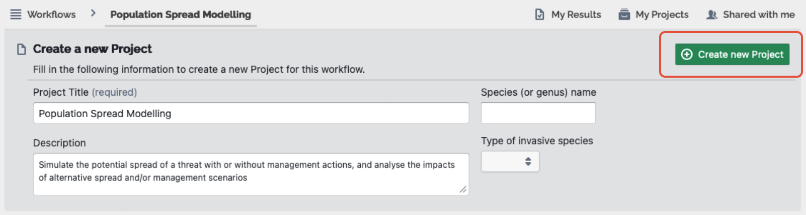
Select the Population Spread Model workflow and then select “Create a new Project” (see screenshot below).
When creating a new population spread model project, users can select an empty template, initially titled “Population Spread Model”, or users can choose from of a range of pre-populated that have been constructed as either examples of the workflow or based on previous case studies (e.g. “Medfly” or “Parkinsonia waterway”).
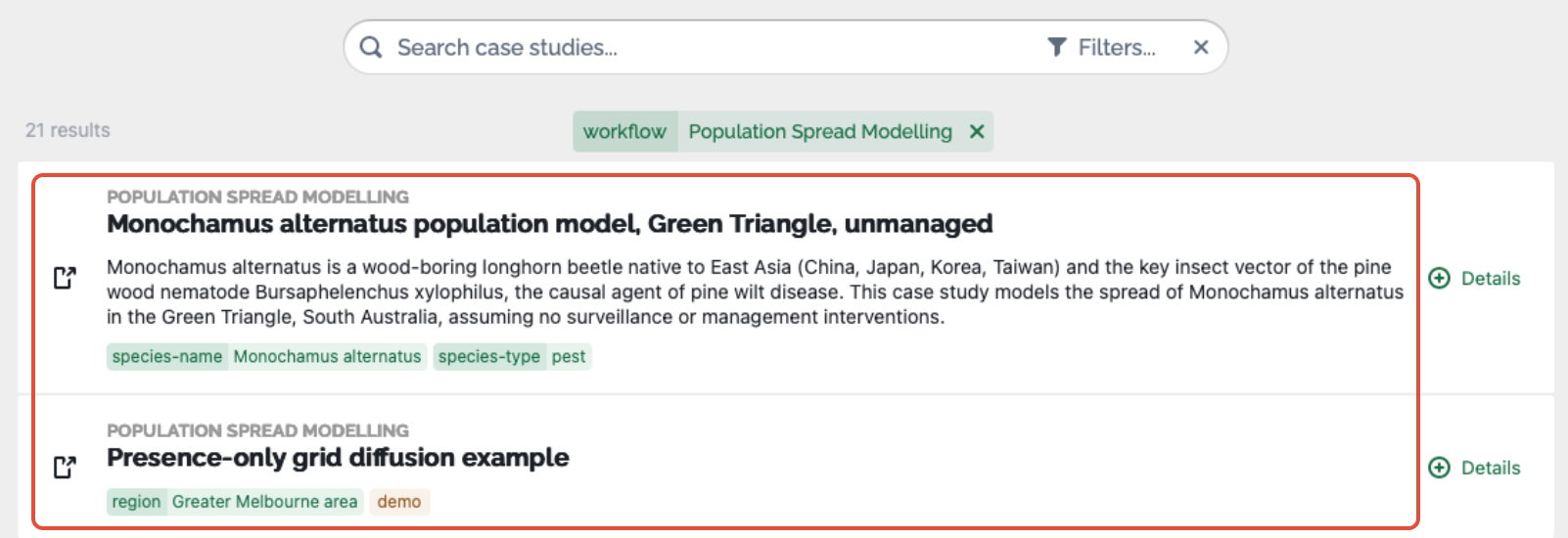
The empty template is ideal for those wishing to create a brand-new population spread model as it contains:
- The basic structure of the population spread model workflow
- No preloaded datasets
By contrast, example templates provide users with the opportunity to see a completed demonstration of how population spread models can be produced, or if based on a real-world case study, how others have attempted to create a model.
Select a template and then give your project an appropriate title. Users can also optionally provide additional descriptive details under the Description, Species name and Species type tabs fields. Project title is the only required field to be completed. These metadata are presently unused but will provide future flexibility in filtering and summarising projects.
Once details have been provided, click the green “Create a new Project” button in the bottom right-hand corner to continue.
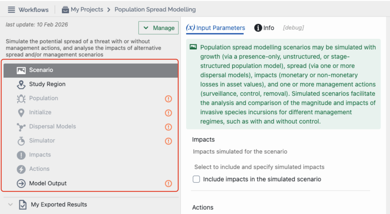
When you start a Population Spread Modelling workflow from an empty template you will be presented with the core elements of the workflow on the left side of the screen – “Scenario”, “Study Region”, “Population”, “Initialize”, “Dispersal Models”, “Simulator”, “Impacts”, “Actions”, and “Model Output”. As you progress through the project, you must address all the steps in the tree with orange exclamation points which indicate steps that require attention. These change to green ticks when complete.
Step 2. Specify the scenario
Population spread modelling scenarios may be simulated with growth, spread, impacts, and one or more management actions (e.g. surveillance, control, removal). Simulated scenarios facilitate the analysis and comparison of the magnitude and impacts of invasive species incursions for different management regimes, such as with and without control. Select the relevant checkboxes to indicate the inclusion of one or more impacts and actions:
- Impacts – include impacts in the simulated scenario
- Ecological impacts
- Social impacts
- Economic impacts
- Actions – include actions in the simulated scenario
- Surveillance actions
- Control actions
- Removal actions
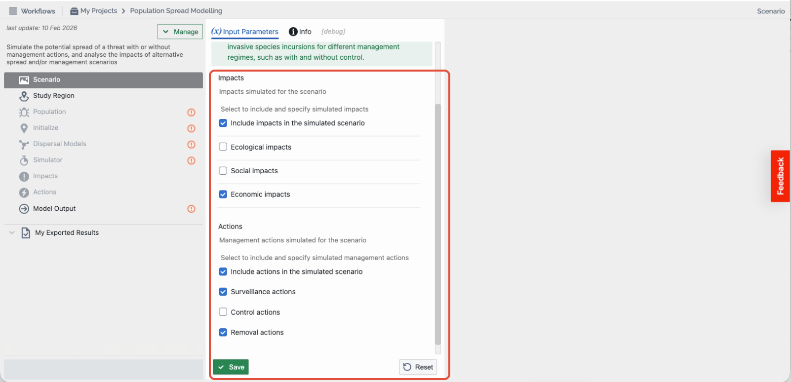
Currently, scenario settings are informational only. In future versions of the platform, these selections may dynamically alter the inclusion of other workflow items or parameters.
Select “Save” if enabled (note that data file selection may autosave your selections).
Step 3. Specify the study region
First, select the model type in the “Study Region” step from the following three options:
- Grid model – Simulate dispersal across a region consisting of a raster of grid cells. Useful for modelling dispersal across landscapes via functionality provided by a wide variety of rasterised data products.
- Network model – Simulate dispersal between a set of interconnected nodes, locations, or patches. Useful when the focus is modelling risk between known nodes (e.g. farms, orchards), and where there is a known risk of movement between nodes.
- Spatially implicit – Simulate dispersal as a spatially implicit area of occupancy that potentially increases over time. Useful for some rapid risk assessments and benefit-cost analyses that do not have, or do not require, detailed information on spatial constraints.
Depending on the model type the user selects, different options will become available.
Next, users specify either:
1. Raster grid model type
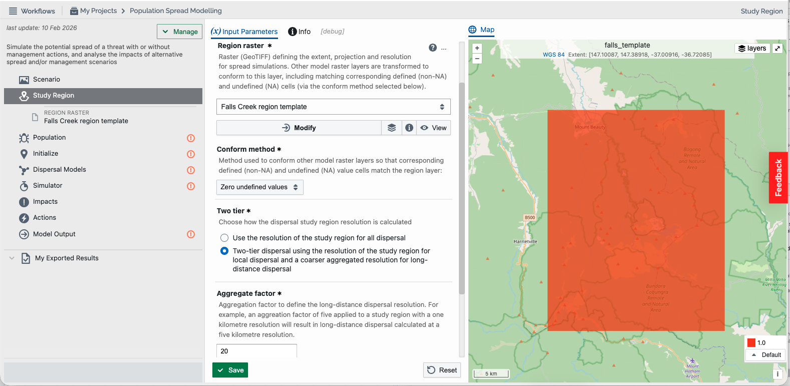
- Region raster (Required): Raster (GeoTIFF) defining the extent, projection and resolution for the population spread model.
- Conform method (Required): Method used to conform other model raster layers so that corresponding defined (non-NA) and undefined (NA) value cells match the region layer, select either:
- Zero undefined values – any cells with undefined (NA) values that do not correspond to undefined (NA) values in the region layer will be set to zero. This default method is useful when available model layers differ in their spatial distribution of defined (non-NA) and undefined (NA) value cells.
- Nearest defined values – Any cells with undefined (NA) values that do not correspond to undefined (NA) values in the region layer will be set to the (mean) value of the nearest cell(s) with defined values. This method is useful for correcting mismatching borders or coastlines, especially those with differing resolutions.
- Two tier (Required): Choose how the dispersal study region resolution is calculated, select either:
- Use the resolution of the study region for all dispersal
This method is suitable for smaller study areas or when computational resources are not a constraint. - Two-tier dispersal using the resolution of the study region for local dispersal and a coarser aggregated resolution for long-distance dispersal
This dispersal approach attempts to optimize computation for large-scale studies by differentiating between local and long-distance dispersal events.
- Use the resolution of the study region for all dispersal
- Aggregation factor (Required when two-tier selected): defines the long-distance dispersal resolution. For example, an aggregation factor of five applied to a study region with a one-kilometre resolution will result in long-distance dispersal calculated at a five-kilometre resolution.
- Inner radius (Required when two-tier selected): the radius (in metres) that defines the boundary between local dispersal, at the study region resolution, and long-distance dispersal at the aggregate resolution.
The Two-tiered dispersal method works by partitioning dispersal events into two types based on distance:
- Local dispersal: Defined by the inner radius parameter, measured in meters. This determines the size of the circle around each occupied cell that retains the original resolution of the study region.
- Long-distance dispersal: Occur beyond the defined inner radius and are simulated using a coarser grid, determined by the aggregation factor.
To illustrate this concept, consider a study region with a 1 km² resolution. If the inner radius is set to 5 km, the model uses the 1 km² cells for dispersal events that occur within the 5 km inner radius. For long-distance dispersal events with an aggregation factor set to 20, aggregated 20 x 20 km (400 km²) cells would be created beyond the inner radius. When a dispersal event extends beyond the inner radius, the model first selects one of these larger 400 km² aggregated cells, then randomly chooses a 1 km² cell within the aggregated cell as the specific dispersal location.
This two-tiered dispersal approach offers several benefits. It significantly reduces computation time for large areas while preserving detailed resolution for local dispersal. It's particularly effective for modelling rare long-distance dispersal events efficiently. Moreover, it allows users to balance computational efficiency with model accuracy by adjusting the inner radius and aggregation factor. This method is especially useful for simulating dispersal over extensive areas or for species with occasional long-distance dispersal events, making it a valuable tool in large-scale ecological and biosecurity studies. By default, when two-tier dispersal is selected, the aggregation factor is set to 20 and the inner radius is set to 5000m.
Select “Save” if enabled (note that data file selection may autosave your selections).
2. Network model type
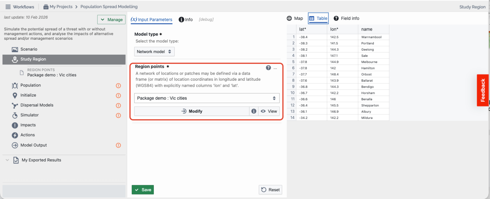
- Region points (Required): Locations or patches may be defined via a CSV table of location coordinates in longitude and latitude (WGS84) with explicitly named columns 'lon' and 'lat'. Auxiliary columns (such as 'name') are also accepted but not used by the model.
Select “Save” if enabled (note that data file selection may autosave your selections).
3. Spatially implicit model type
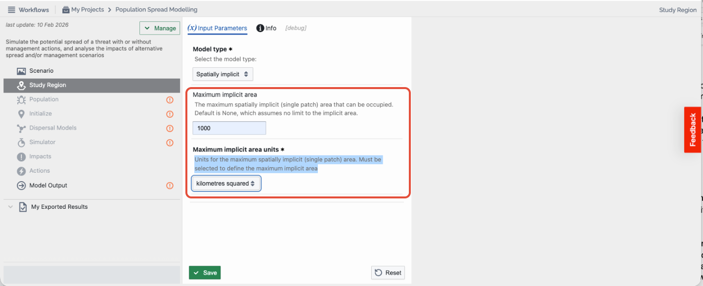
- Maximum implicit area (Optional): The maximum spatially implicit (single patch) area that can be occupied. Default is none, which assumes no limit to the implicit area.
- Maximum implicit area units (Required when maximum implicit area is selected): Units for the maximum spatially implicit (single patch) area. Select either 'metres squared' or 'kilometres squared'. Must be selected to define the maximum implicit area.
Note: If users do not specify a maximum implicit area, the platform will assume there is no limit to the area that can be occupied. Depending on the spread dynamics specified, this can result in unrealistic estimates of area occupied or population sizes, and in extreme cases may reach population sizes beyond integer data limits. As such, we STRONGLY RECOMMEND users specify a maximum implicit area.
Select “Save” if enabled (note that data file selection may autosave your selections).
Step 4. Specify the population
The presence/absence or size of a population at a location is a critical factor in Population Spread Modelling. Biosecurity Commons provides users with the ability to use three types of population models within their spread models. Firstly, users specify the population model type from either:
- Presence-only: This is the simplest option. It ignores population structure and produces a binary output indicating only the presence and absence of a threat.
- Unstructured: An unstructured population focuses on modelling a population by considering the average population's intrinsic growth rate.
- Stage-structured: A stage-structured model requires users to specify a stage or aged-based transition matrix. This indicates how many new individuals (or offspring) will be added to the population at each time step, given species reproductive rates, and the probability of surviving, or transitioning to subsequent stages, at each simulation time step.
Depending on the population type the user selects, different options will become available. Next, users specify either:
1. Presence-only population model
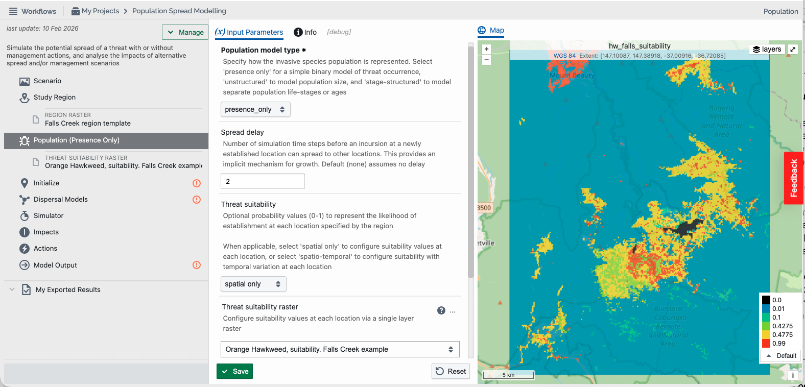
- Spread delay (Optional:grid or network models): Allows users to specify the number of simulation time steps an occupied location must wait before spread can occur. This can be useful for certain threats such as weeds that must reach reproductive maturity before they can spread.
- Threat suitability (Optional: grid and network models): A raster (grid model) or point data (network model) with values between 0 and 1 that specify the suitability (or establishment likelihood) of each cell/point location and/or time step. This parameter is useful to prevent or reduce the establishment when the invasive species spread to locations that are otherwise deemed unsuitable or have low suitability. Threat suitability can be based on both abiotic and biotic factors (e.g. see Risk Mapping) or a subset of these. If not provided, suitability is assumed to be uniform across grid cells or point locations. Threat suitability may be configured with or without temporal variation via selection:
- Spatial only – to configure (static) suitability values at each location, defined dependent on the study region model type selected in Step 3:
- Grid model – a raster grid (GeoTIFF)
- Network model – a CSV file having aligned ‘lon’, ‘lat’, and ‘suitability’ columns
- Spatio-temporal – to configure suitability with temporal variation at each location, defined dependent on the study region model type selected in Step 3:
- Grid model – a multi-layer raster grid (GeoTIFF) with sequential temporal layers
- Network model – a CSV file having aligned ‘lon’, ‘lat’, and sequential columns for temporal suitability labelled ‘suitability_1’, ‘suitability_2’, etc.
- Spatial only – to configure (static) suitability values at each location, defined dependent on the study region model type selected in Step 3:
The number of raster grid layers or CSV columns utilised for temporal variation should either coincide with the number of simulation time steps (see Step 7), or form a cyclic pattern (e.g. 12 rows for seasonal variation with monthly time steps).
- Threat suitability raster (grid) or data (network): select the raster grid or data CSV file via existing project results or stored datasets or upload a file to the platform. Existing data may also be altered via toolbox functionality prior to being used by the model.
- Suitability dynamically impacted by incursion (grid & network models): threat suitability may also be dynamically impacted by an incursion. Select the checkbox to link suitability to dynamic impacts of a resource or asset that the threat utilises (e.g. plantation), then configure dynamic impacts in the Impacts section.
Select “Save” if enabled (note that data file selection may autosave your selections).
2. Unstructured population model
- Growth (Required): Finite rate of population growth or lambda. For example, a growth rate of 1.2 will increase the population size by 20% at each time-step (or less when the population is capacity-limited – see below). Growth may be configured with or without spatial and/or temporal variation via selection:
- Single value (all models) – to configure a uniform value across space and time
- Spatial only (grid & network models) – to configure (static) values at each location, defined dependent on the study region model type selected in Step 3:
- Grid model – a raster grid (GeoTIFF)
- Network model – a CSV file having aligned ‘lon’, ‘lat’, and ‘growth’ columns
- Temporal [only] (all models) – to configure variability across time, defined via a CSV file with a temporal ‘growth’ column
- Spatio-temporal (grid & network models) – to configure variability across space and time, defined dependent on the study region model type selected in Step 3:
- Grid model – a multi-layer raster grid (GeoTIFF) with sequential temporal layers
- Network model – a CSV file having aligned ‘lon’, ‘lat’, and sequential columns for temporal growth labelled ‘growth_1’, ‘growth_2’, etc.
The number of raster grid layers or CSV rows/columns utilised for temporal variation should either coincide with the number of simulation time steps (see Step 7) or form a cyclic pattern (e.g. 12 rows for seasonal variation with monthly time steps).
- Growth raster (grid) or data (network, temporal) – (Required when growth is variable, i.e. not a single value): select the raster grid or data CSV file via existing project results or stored datasets or upload a file to the platform. Existing data may also be altered via toolbox functionality prior to being used by the model.
- Threat suitability (Optional: grid and network models): A raster (grid model) or point data (network model) with values between 0 and 1 that specify the suitability (or establishment likelihood) of each cell/point location and/or time step. This parameter is useful to prevent or reduce the establishment when the invasive species spread to locations that are otherwise deemed unsuitable or have low suitability. Threat suitability can be based on both abiotic and biotic factors (e.g. see Risk Mapping) or a subset of these. If not provided, suitability is assumed to be uniform across grid cells or point locations. Threat suitability may be configured with or without temporal variation via selection:
- Spatial only – to configure (static) suitability values at each location, defined dependent on the study region model type selected in Step 3:
- Grid model – a raster grid (GeoTIFF)
- Network model – a CSV file having aligned ‘lon’, ‘lat’, and ‘suitability’ columns
- Spatio-temporal – to configure suitability with temporal variation at each location, defined dependent on the study region model type selected in Step 3:
- Grid model – a multi-layer raster grid (GeoTIFF) with sequential temporal layers
- Network model – a CSV file having aligned ‘lon’, ‘lat’, and sequential columns for temporal suitability labelled ‘suitability_1’, ‘suitability_2’, etc.
- Spatial only – to configure (static) suitability values at each location, defined dependent on the study region model type selected in Step 3:
The number of raster grid layers or CSV columns utilised for temporal variation should either coincide with the number of simulation time steps (see Step 7), or form a cyclic pattern (e.g. 12 rows for seasonal variation with monthly time steps).
- Threat suitability raster (grid) or data (network): select the raster grid or data CSV file via existing project results or stored datasets or upload a file to the platform. Existing data may also be altered via toolbox functionality prior to being used by the model.
- Suitability dynamically impacted by incursion (grid & network models): threat suitability may also be dynamically impacted by an incursion. Select the checkbox to link suitability to dynamic impacts of a resource or asset that the threat utilises (e.g. plantation), then configure dynamic impacts in the Impacts section.
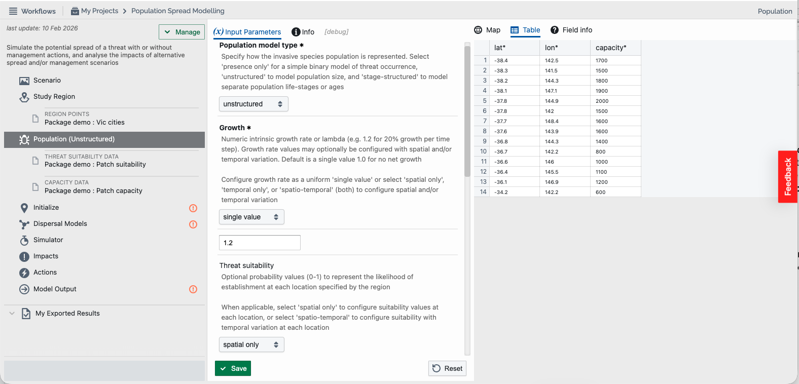
- Carrying Capacity (Optional): carrying capacity defines the maximum sustainable population size at a given location or per unit area. For grid-based or network models, capacity is specified across locations. Note: often carrying capacity is assumed to be proportional to the suitability of a location. For example, if the carrying capacity in a location with perfect suitability (i.e. score = 1) is 5,000, then the carrying capacity in a cell with a suitability score of 0.5 = 2,500. The platform is agnostic as to how users derive their estimates of carrying capacity. Grid-based or network-based capacity may be configured with or without temporal variation via selection:
- Spatial only (grid & network models) – to configure (static) suitability values at each location, defined dependent on the study region model type selected in Step 3:
- Grid model – a raster grid (GeoTIFF)
- Network model – a CSV file having aligned ‘lon’, ‘lat’, and ‘capacity’ columns
- Spatio-temporal (grid & network models) – to configure suitability with temporal variation at each location, defined dependent on the study region model type selected in Step 3:
- Grid model – a multi-layer raster grid (GeoTIFF) with sequential temporal layers
- Network model – a CSV file having aligned ‘lon’, ‘lat’, and sequential columns for temporal capacity labelled ‘capacity_1’, ‘capacity_2’, etc.
- Spatial only (grid & network models) – to configure (static) suitability values at each location, defined dependent on the study region model type selected in Step 3:
The number of raster grid layers or CSV columns utilised for temporal variation should either coincide with the number of simulation time steps (see Step 7), or form a cyclic pattern (e.g. 12 layers/columns for seasonal variation with monthly time steps).
Spatially implicit capacity may be configured per unit area with or without temporal variation via selection:
- Single value (spatially implicit models) – to configure a value
- Temporal (spatially implicit models) – to configure variability across time, defined via a CSV file with a temporal ‘suitability’ column. The number of CSV rows utilised for temporal variation should either coincide with the number of simulation time steps (see Step 7), or form a cyclic pattern (e.g. 12 rows for seasonal variation with monthly time steps).
The area unit used when specifying capacity for spatially implicit models also needs to be selected.
- Capacity raster (grid) or data (network, spatially implicit - temporal): select the raster grid or data CSV file via existing project results or stored datasets or upload a file to the platform. Existing data may also be altered via toolbox functionality prior to being used by the model.
- Capacity area unit (Required if carrying capacity is configured for spatially implicit unstructured or staged structured models):
- Metres squared
- Kilometres squared
- Maximum area (i.e. maximum implicit area when defined in the study region)
- Capacity dynamically impacted by incursion (grid, network, & spatially implicit): Capacity may also be dynamically impacted by an incursion. Select the checkbox to link carrying capacity to dynamic impacts of a resource or asset that the threat utilises (e.g. plantation), then configure dynamic impacts in the Impacts section.
Select “Save” if enabled (note that data file selection may autosave your selections).
3. Stage-structured population model
- Growth Matrix (Required: grid, network, & spatially implicit models): A transition matrix by age or stage that describes reproductive rates, stage transition likelihoods and same-stage survival likelihoods (see example below).
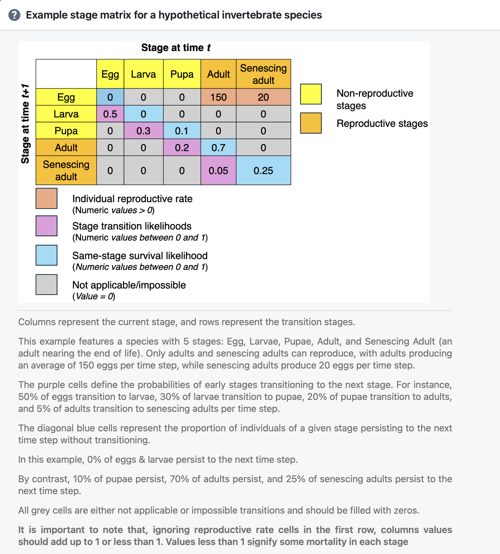
The size of the matrix may be appropriately adjusted. Labels representing the stage or age levels may also be added to the rows of the matrix.
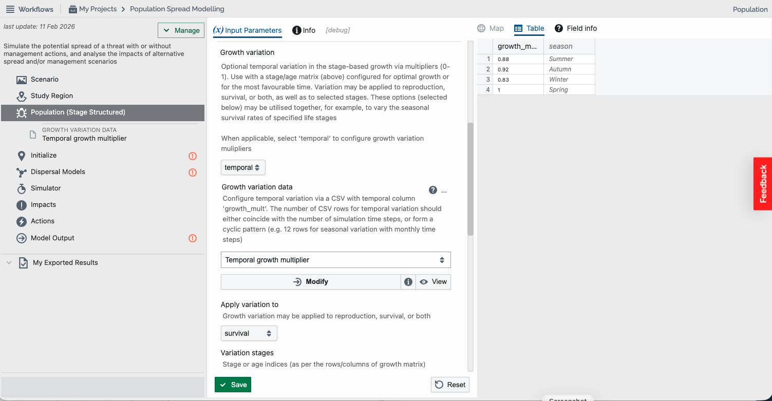
- Growth variation (Optional): Optional temporal variation in the stage-based growth via multipliers (0-1), whereby 0 inhibits growth and values less than 1 cause a reduction in growth. Use with a stage/age matrix (above) configured for optimal growth or for the most favourable time. Variation may be applied to reproduction, survival, or both, as well as to selected stages. These options (selected below) may be utilised together, for example, to vary the seasonal survival rates of specified life stages. Growth variation may be applied with spatial and/or temporal variation via selection:
- Spatial only (grid & network models) – to configure (static) values at each location, defined dependent on the study region model type selected in Step 3:
- Grid model – a raster grid (GeoTIFF)
- Network model – a CSV file having aligned ‘lon’, ‘lat’, and ‘growth_mult’ columns
- Temporal [only] (all models) – to configure a variability multiplier across time, defined via a CSV file with a temporal ‘growth_mult’ column
- Spatio-temporal (grid & network models) – to configure a variability multiplier across space and time, defined dependent on the study region model type selected in Step 3:
- Grid model – a multi-layer raster grid (GeoTIFF) with sequential temporal layers
- Network model – a CSV file having aligned ‘lon’, ‘lat’, and sequential columns for temporal growth labelled ‘growth_mult_1’, ‘growth_mult_2’, etc.
- Spatial only (grid & network models) – to configure (static) values at each location, defined dependent on the study region model type selected in Step 3:
The number of raster grid layers or CSV rows/columns utilised for temporal variation should either coincide with the number of simulation time steps (see Step 7) or form a cyclic pattern (e.g. 12 rows for seasonal variation with monthly time steps).
- Growth variation raster (grid) or data (network, temporal) – (Required when growth variation is selected): select the raster grid or data CSV file via existing project results or stored datasets or upload a file to the platform. Existing data may also be altered via toolbox functionality prior to being used by the model.
- Apply variation to (when growth variation is selected): select what aspects of the staged growth the variation (multiplier) should be applied to, from:
- Reproduction
- Survival
- Both (reproduction & survival)
- Variation stages (when growth variation is selected): Users can specify which life-stages/ages are applicable for growth variation. A checkbox will appear for each stage/age (i.e. column) specified in the growth matrix for users to select. If none are selected, all stages are assumed to be applicable.
- Threat suitability (Optional: grid and network models): A raster (grid model) or point data (network model) with values between 0 and 1 that specify the suitability (or establishment likelihood) of each cell/point location and/or time step. This parameter is useful to prevent or reduce the establishment when the invasive species spread to locations that are otherwise deemed unsuitable or have low suitability. Threat suitability can be based on both abiotic and biotic factors (e.g. see Risk Mapping) or a subset of these. If not provided, suitability is assumed to be uniform across grid cells or point locations. Threat suitability may be configured with or without temporal variation via selection:
- Spatial only – to configure (static) suitability values at each location, defined dependent on the study region model type selected in Step 3:
- Grid model – a raster grid (GeoTIFF)
- Network model – a CSV file having aligned ‘lon’, ‘lat’, and ‘suitability’ columns
- Spatio-temporal – to configure suitability with temporal variation at each location, defined dependent on the study region model type selected in Step 3:
- Grid model – a multi-layer raster grid (GeoTIFF) with sequential temporal layers
- Network model – a CSV file having aligned ‘lon’, ‘lat’, and sequential columns for temporal suitability labelled ‘suitability_1’, ‘suitability_2’, etc.
- Spatial only – to configure (static) suitability values at each location, defined dependent on the study region model type selected in Step 3:
The number of raster grid layers or CSV columns utilised for temporal variation should either coincide with the number of simulation time steps (see Step 7), or form a cyclic pattern (e.g. 12 rows for seasonal variation with monthly time steps).
- Threat suitability raster (grid) or data (network): select the raster grid or data CSV file via existing project results or stored datasets or upload a file to the platform. Existing data may also be altered via toolbox functionality prior to being used by the model.
- Suitability dynamically impacted by incursion (grid & network models): threat suitability may also be dynamically impacted by an incursion. Select the checkbox to link suitability to dynamic impacts of a resource or asset that the threat utilises (e.g. plantation), then configure dynamic impacts in the Impacts section.
- Carrying Capacity (Optional): carrying capacity defines the maximum sustainable population size at a given location or per unit area. For grid-based or network models, capacity is specified across locations. Note: often carrying capacity is assumed to be proportional to the suitability of a location. For example, if the carrying capacity in a location with perfect suitability (i.e. score = 1) is 5,000, then the carrying capacity in a cell with a suitability score of 0.5 = 2,500. The platform is agnostic as to how users derive their estimates of carrying capacity. Grid-based or network-based capacity may be configured with or without temporal variation via selection:
- Spatial only (grid & network models) – to configure (static) suitability values at each location, defined dependent on the study region model type selected in Step 3:
- Grid model – a raster grid (GeoTIFF)
- Network model – a CSV file having aligned ‘lon’, ‘lat’, and ‘capacity’ columns
- Spatio-temporal (grid & network models) – to configure suitability with temporal variation at each location, defined dependent on the study region model type selected in Step 3:
- Grid model – a multi-layer raster grid (GeoTIFF) with sequential temporal layers
- Network model – a CSV file having aligned ‘lon’, ‘lat’, and sequential columns for temporal capacity labelled ‘capacity_1’, ‘capacity_2’, etc.
- Spatial only (grid & network models) – to configure (static) suitability values at each location, defined dependent on the study region model type selected in Step 3:
The number of raster grid layers or CSV columns utilised for temporal variation should either coincide with the number of simulation time steps (see Step 7), or form a cyclic pattern (e.g. 12 layers/columns for seasonal variation with monthly time steps).
Spatially implicit capacity may be configured per unit area with or without temporal variation via selecting:
- Single value (spatially implicit models) – to configure a value
- Temporal (spatially implicit models) – to configure variability across time, defined via a CSV file with a temporal ‘suitability’ column. The number of CSV rows utilised for temporal variation should either coincide with the number of simulation time steps (see Step 7), or form a cyclic pattern (e.g. 12 rows for seasonal variation with monthly time steps).
The area unit used when specifying capacity for spatially implicit models also needs to be selected.
- Capacity raster (grid) or data (network, spatially implicit - temporal): select the raster grid or data CSV file via existing project results or stored datasets or upload a file to the platform. Existing data may also be altered via toolbox functionality prior to being used by the model.
- Capacity area unit (Required if carrying capacity is configured for spatially implicit unstructured or staged structured models):
- Metres squared
- Kilometres squared
- Maximum area (i.e. maximum implicit area when defined in the study region)
- Capacity dynamically impacted by incursion (grid, network, & spatially implicit): Capacity may also be dynamically impacted by an incursion. Select the checkbox to link carrying capacity to dynamic impacts of a resource or asset that the threat utilises (e.g. plantation), then configure dynamic impacts in the Impacts section.
- Capacity Stages (Optional: stage-structured models): Users can specify which life-stages/ages are applicable for capacity-limited growth (and survival). For example, the capacity, or limit to the number of plants that can occupy each location, usually only needs to consider the later growth stages, and is generally not affected by the number of seeds or seedlings. A checkbox will appear for each stage/age (i.e. column) specified in the growth matrix for users to select. If none are selected, all stages are assumed to be applicable.
When you have finished specifying a population model and its parameters, click the green “Save” button and move to the Initialize step in the tree.
Step 5. Configure the model initialization
The Initialize section allows users to specify the starting conditions in which to simulate spread. Again, how this section is specified is dependent on what was selected in the previous two steps (i.e. the selected model type and population type).
If a spatially implicit model type has been selected with a presence-only population type, then a population is assumed to be present, and as such, the Initialize section requires no input from the user. Other combinations of model and population types require user input as follows:
First, select the Initializer type in the “Initialize” step from the following options:
For grid & network models:
- Initial values – assign the initial population at each location
- Random location – select a random initial location via relative weights
For spatially implicit models:
- Initial size – assign the initial population size
- Random (Poisson mean) – generate a random initial incursion sampled from a Poisson distribution
Depending on the initializer type the user selects, different options will become available. Next, users specify either:
1.1. Initial values (grid & network models)
- Initial layer type (Required: grid models): The initial layer may be defined in two ways, select either:
- Use an existing population values raster – then specify:
- Initializer raster (Required): A raster grid (GeoTIFF) defining the initial population distribution.
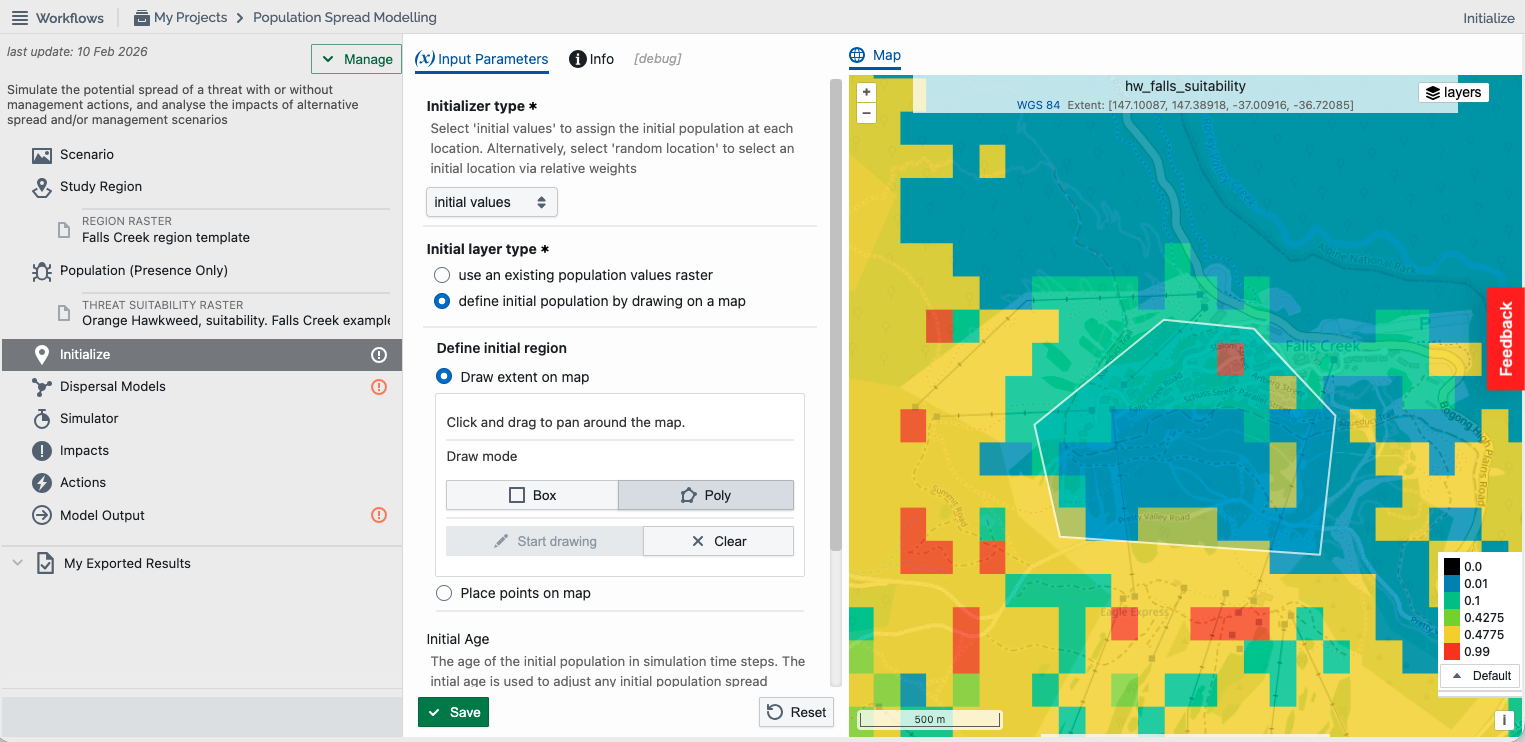
- Define initial population by drawing on a map – then specify:
- Define initial region (Required): Select either:
- Draw extent on map – the user may draw a rectangle or polygon to define the initial area of occupancy
- Place points on map – the user may draw one or more points to define the initial occupancy locations
- Population size (Required: unstructured & stage-structured populations): The total initial population that will be distributed over the defined initial area/locations.
- Initializer data (Required: network models): The initial population values at each location defined via a CSV table with a row for each location and a single column 'population'.
- Initial age (Optional: presence-only & stage-structured populations): The age of the initial population in simulation time steps. The initial age is used to adjust any initial population spread delays in presence-only populations, or determine which stages are initially present in stage-based models. Specify either:
- As a ‘single value’ for the entire study
- Vary values ‘across locations’ via a raster grid (GeoTIFF)
- First occupancy stages (Required: stage-structured populations): Indicate which life-stages/ages are initially present (at first occupancy when age = 0 if initial age is specified). A checkbox will appear for each stage/age (i.e. column) specified in the growth matrix for users to select. If none are selected, all stages are assumed to be applicable.
Select “Save” if enabled (note that data file selection may autosave your selections).
1.2. Random location (grid & network models)
- Initializer raster (Required: grid models): A raster grid (GeoTIFF) defining the incursion weightings or arrival probabilities at each spatial location.
- Initializer data (Required: network models): The incursion weightings or arrival probabilities at each location defined via a CSV table with a row for each location and a single column 'weights'.
- Incursion mean (Required: unstructured & stage-structured populations): Numeric mean population size for incursion locations. The population size is sampled from the Poisson distribution for each incursion location.
- Incursion stages (Required: stage-structured populations): Indicate which life-stages/ages are applicable for random incursions. A checkbox will appear for each stage/age (i.e. column) specified in the growth matrix for users to select. If none are selected, all stages are assumed to be applicable.
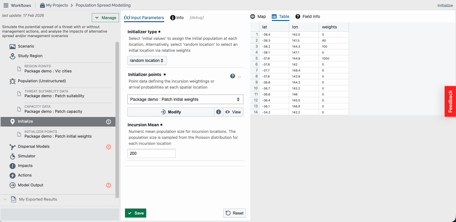
Select “Save” if enabled (note that data file selection may autosave your selections).
2.1. Initial size (spatially implicit models)
- Initial population size (Required; unstructured & stage-structured populations): The number of individuals initially present in each model simulation.
- Initial stages (Required: stage-structured populations): Indicate which life-stages/ages are initially present. A checkbox will appear for each stage/age (i.e. column) specified in the growth matrix for users to select. If none are selected, all stages are assumed to be applicable.
2.2. Random – Poisson mean (spatially implicit models)
- Incursion mean (Optional:grid or network models): The mean initial population incursion size. The initial number of individuals is sampled from the Poisson distribution (with the specified mean) for each model simulation.
- Initial stages (Required: stage-structured populations): Indicate which life-stages/ages are initially present. A checkbox will appear for each stage/age (i.e. column) specified in the growth matrix for users to select. If none are selected, all stages are assumed to be applicable.
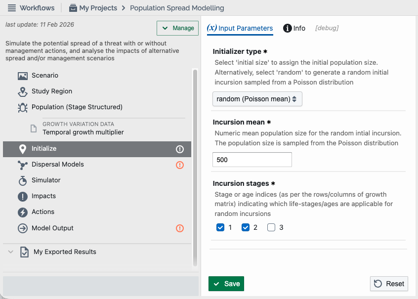
When you have finished, click the green “Save” button and move to the “Dispersal Models” step in the tree.
Step 6. Specify the dispersal model(s)
Threat dispersal or spread can be modelled using many mathematical functions. Biosecurity Commons has attempted to consolidate these into a handful of generic functions that can incorporate a wide range of processes and constraints. These include:
- Kernel Dispersal (grid & network models; all population models): A highly flexible method allowing users to disperse risk as a function of distance decay, direction, spread event likelihoods, attractors, and spatial constraints.
- Dispersal Diffusion (grid models only; all populations models): A simple method for modelling diffusive spread processes as a function of an average spread rate, directional weighting, attractors, and spatial constraints.
- Dispersal Gravity (network models only; all population models): Models the dispersion of risk using gravity-like diffusion between locations based on specific inter-location attraction, the strength of which decays with increasing distance between locations.
- Radial Diffusion (spatially implicit models with presence-only population models): Models spatial-implicit area as a function of radial diffusion of threat occupancy.
- Area Spread (spatially implicit models with unstructured or stage-structured population models): Models spread in (implicit) occupied area, whereby the occupied area increases proportionally to the size of the population, which may be capacity limited. When the population is capacity-limited and the maximum implicit area is specified, the time series graph of the total population size, and thus area occupied, follows a typical “S-curve”.
- Reaction-Diffusion (spatially implicit models with unstructured or stage-structured population models): A reaction-diffusion dispersal model is a mathematical framework that describes the spatial and temporal spread of a population by combining two key processes: reaction (population growth) and diffusion (spatial spread). In this model, the change in population density over time is governed by the interplay of intrinsic growth rate (r), carrying capacity (K), and diffusion rate (D). Typically, lower diffusion rates result in lower population growth, since the implicit space available to populations having capacity-limited growth does not expand as quickly as models with higher diffusion rates.
To add a dispersal model, select “Add New Input” in the Dispersal Models section of the tree:
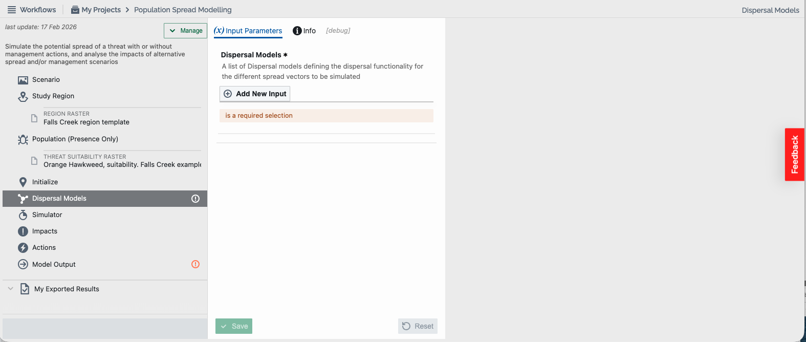
The functions available to the user depend on the model type and population models specified. For example, if a user has specified a grid model with an unstructured population model, then the options available for selection will be Kernel Dispersal & Dispersal Diffusion.
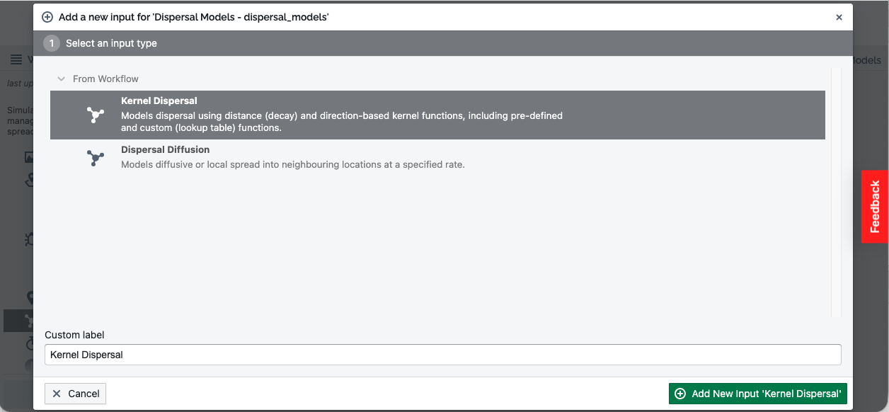
For spatially explicit (grid and network) models, multiple dispersal functions can be specified by the user (each added separately), whereby each function may represent a different mode of spread. For example, a user may specify a Dispersal Diffusion function to simulate localised/natural spread and multiple Kernel Dispersal functions to simulate spread caused by different vectors (e.g. human movement, wind dispersal etc.). However, only one dispersal function may be applied to spatially implicit models.
1. Kernel Dispersal
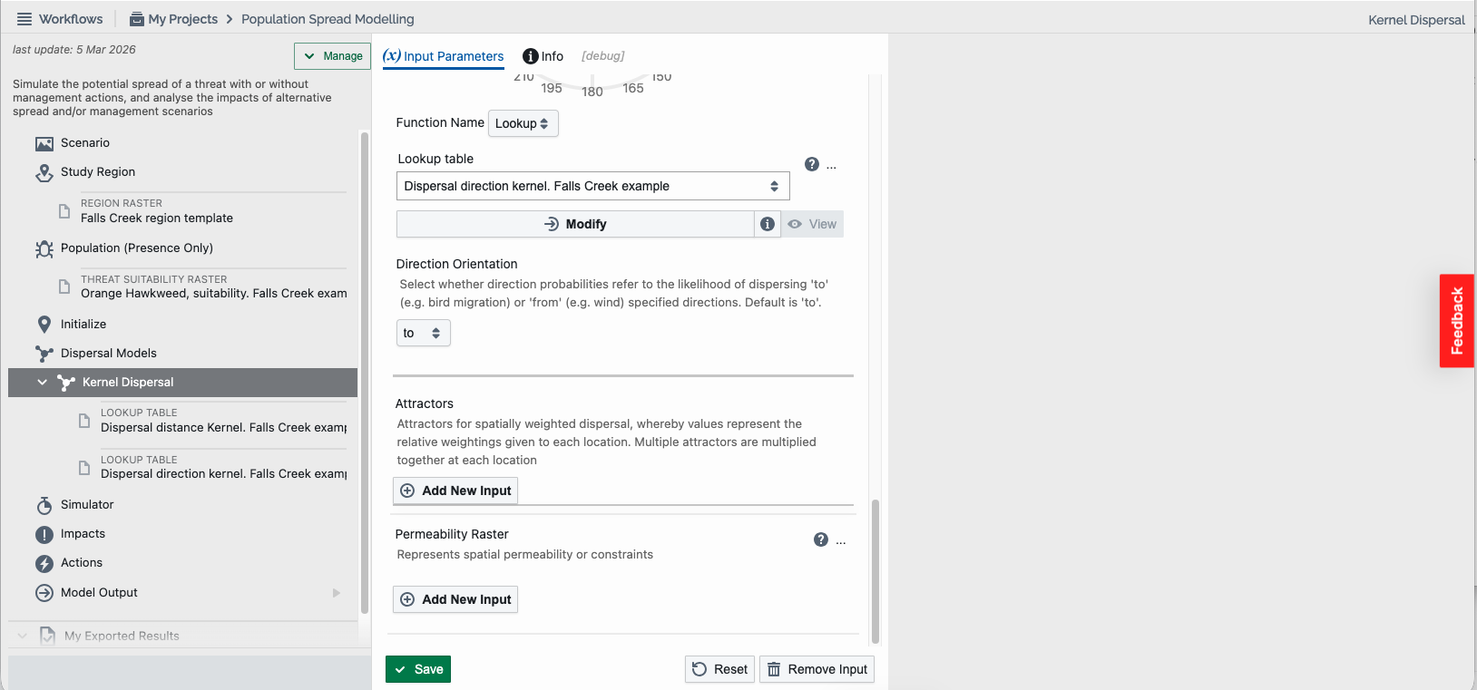
When users select Kernal Dispersal, a new sub step appears in the tree and multiple modification options will become available (see screenshot below). Kernel dispersal models can only be used in spatially explicit contexts (i.e. grid and network models) and are thus not available for spatially implicit models.
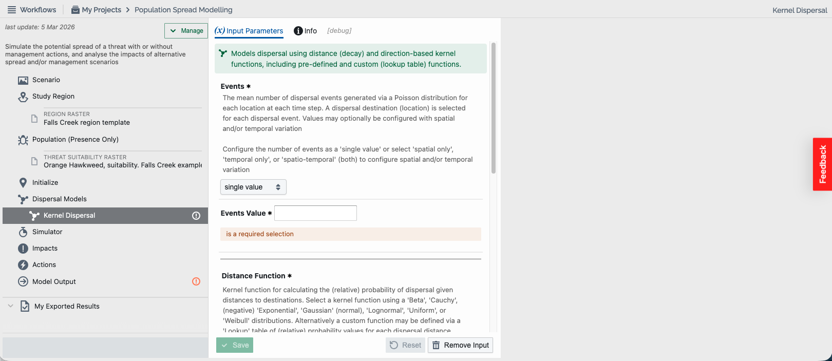
Kernel dispersal contains a range of required and optional fields that can be filled in. These include:
- Dispersal stages (Required for stage-structured populations only): Indicate which life-stages/ages disperse. A checkbox will appear for each stage/age (i.e. column) specified in the growth matrix for users to select. If none are selected, all stages are assumed to be applicable.
- Proportion (Required for unstructured or stage-structured populations): A parameter that specifies the proportion of the population at each location that disperses at each simulation time-step. Proportion may be configured with or without spatial and/or temporal variation via selection:
- Single value (all models) – to configure a uniform value across space and time
- Spatial only (grid & network models) – to configure (static) values at each location, defined dependent on the study region model type selected in Step 3:
- Grid model – a raster grid (GeoTIFF)
- Network model – a CSV file having aligned ‘lon’, ‘lat’, and ‘proportion’ columns
- Temporal [only] (all models) – to configure variability across time, defined via a CSV file with a temporal ‘proportion’ column
- Spatio-temporal (grid & network models) – to configure variability across space and time, defined dependent on the study region model type selected in Step 3:
- Grid model – a multi-layer raster grid (GeoTIFF) with sequential temporal layers
- Network model – a CSV file having aligned ‘lon’, ‘lat’, and sequential columns for temporal growth labelled ‘proportion_1’, ‘proportion_2’, etc.
The number of raster grid layers or CSV rows/columns utilised for temporal variation should either coincide with the number of simulation time steps (see Step 7) or form a cyclic pattern (e.g. 12 rows for seasonal variation with monthly time steps).
- Proportion raster (grid) or data (network, temporal) – (Required when proportion is variable, i.e. not a single value): select the raster grid or data CSV file via existing project results or stored datasets or upload a file to the platform. Existing data may also be altered via toolbox functionality prior to being used by the model.
- Events (Required for presence-only models; Optional for unstructured or stage-structured populations): A parameter that specifies the mean number of dispersal events for each location at each time step. Numbers are generated using a Poisson distribution. Events may be configured with or without spatial and/or temporal variation via selection:
- Single value (all models) – to configure a uniform value across space and time.
- Spatial only (grid & network models) – to configure (static) values at each location, defined dependent on the study region model type selected in Step 3:
- Grid model – a raster grid (GeoTIFF)
- Network model – a CSV file having aligned ‘lon’, ‘lat’, and ‘events’ columns
- Temporal [only] (all models) – to configure variability across time, defined via a CSV file with a temporal ‘events’ column
- Spatio-temporal (grid & network models) – to configure variability across space and time, defined dependent on the study region model type selected in Step 3:
- Grid model – a multi-layer raster grid (GeoTIFF) with sequential temporal layers
- Network model – a CSV file having aligned ‘lon’, ‘lat’, and sequential columns for temporal growth labelled ‘events_1’, ‘events_2’, etc.
The number of raster grid layers or CSV rows/columns utilised for temporal variation should either coincide with the number of simulation time steps (see Step 7) or form a cyclic pattern (e.g. 12 rows for seasonal variation with monthly time steps).
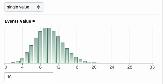
- Events value (Required when the number of events is a single value): When entered, the Poisson distribution of single-value events will be displayed graphically.
- Events raster (grid) or data (network, temporal) – (Required when the number of events is variable, i.e. not a single value): select the raster grid or data CSV file via existing project results or stored datasets or upload a file to the platform. Existing data may also be altered via toolbox functionality prior to being used by the model.
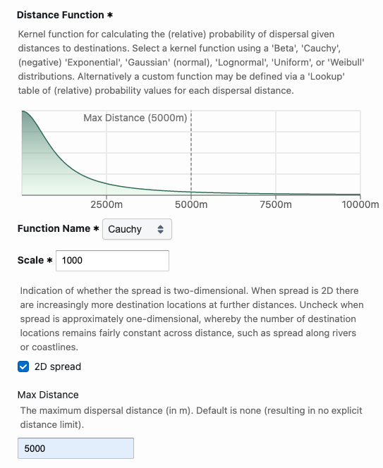
- Distance function (Required): A kernel function describing the relative likelihood a spread event will travel a particular distance. The platform provides users with a wide range of commonly used distribution functions that they can parameterize and visualize on the platform. The predefined distribution functions
include:- Beta (params: Alpha, Beta, Upper distance limit)
- Cauchy (params: Scale)
- Negative exponential (params: Mean)
- Gaussian (params: Standard Deviation)
- Lognormal (params: Mean, Standard Deviation)
- Weibull (params: Shape, Scale)
- Uniform (params: Lower, Upper)
Once configured a plot of the parameterised distribution will be displayed for convenience (see example below).
Alternatively, users may define their own custom functions via lookup tables:
- Lookup – Provides the ability for users to import their own custom kernel via a tabular CSV file. This file requires two columns: ‘distance' and ‘probability’. Data should be ordered from shortest to longest distance and all distances must contain a probability. When users add the CSV file it will appear as a chart (see screenshot below).
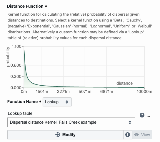
The tabular values may also be viewed via the data tree item.
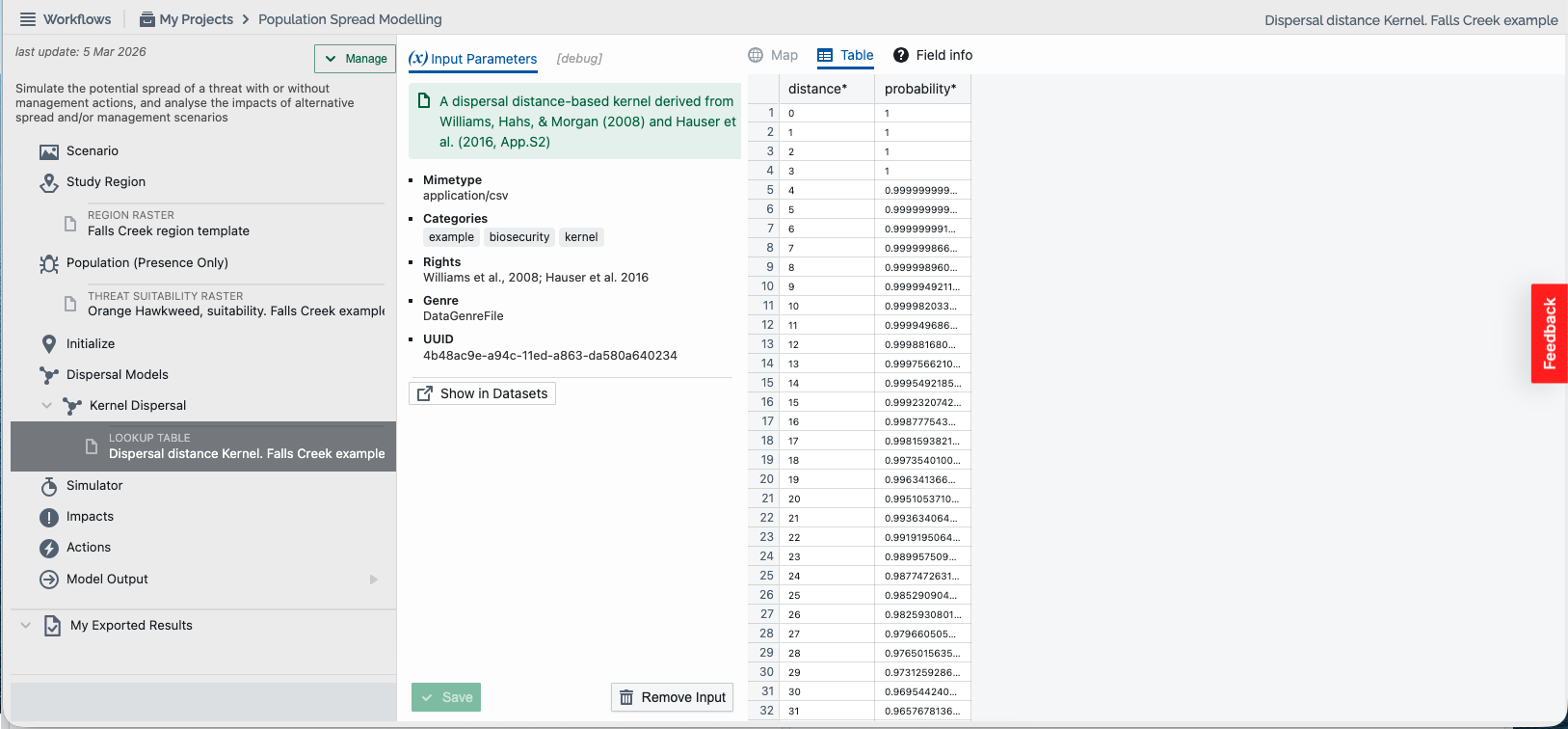
- 2D spread (Required – default is checked): Indication of whether the spread is two-dimensional. When spread is 2D there are increasingly more destination locations at further distances. Uncheck when spread is approximately one-dimensional, whereby the number of destination locations remains approximately constant across distance, such as spread along rivers or coastlines.
- Max distance (Optional): The maximum dispersal distance (in m). Default is none (resulting in no explicit distance limit).
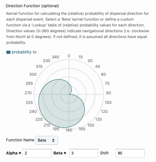
- Direction function (Optional): Specifies the probability of dispersal events moving in one direction over another. By default, dispersal events can move in any direction with equal probability. Alternatively, users may specify a directional spread by selecting Function name under Direction function, and choose between:
- Beta (params: Beta, Alpha, Shift) – A simple beta distribution with an optional “Shift” parameter, which can be used to rotate the Beta curve (0-360 degrees). Specifying the parameters of this distribution will automatically be visualised for user interpretation.
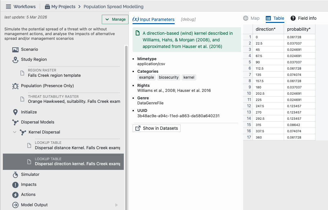
- Lookup – Provides the ability for users to import their own custom directional kernel via a CSV file. This file requires two columns: ‘direction’ and ‘probability’. Data should be ordered from smallest to largest direction (measured in degrees), and all directions must contain a probability. When users add the CSV file it will appear as a chart (see screenshot below).
- Beta (params: Beta, Alpha, Shift) – A simple beta distribution with an optional “Shift” parameter, which can be used to rotate the Beta curve (0-360 degrees). Specifying the parameters of this distribution will automatically be visualised for user interpretation.
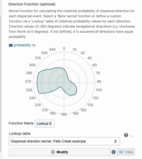
The tabular values may also be viewed via the data tree item.
- Direction orientation (Optional): Select whether direction probabilities refer to the likelihood of dispersing 'to' (e.g. bird migration) or 'from' (e.g. wind) specified directions. Default is 'to'.
- Attractors (Optional) - Users can specify one or multiple attractors that can be used to inform the relative weightings to be applied to each location during a spread event. Attractors are weightings for probability for destination locations.
- For grid models attractors are specified via raster layers.
- For network models attractors are specified as location specific relative weightings for each location/node in a tabular format, configured via a CSV file with headers containing coordinate columns 'lon' and 'lat', and an 'attractor' column with weighting values. Various attributes can be used to inform attractors, such as habitat suitability, abundance of host/food source, or other landscape variables that may attract vectors of risk material movement (e.g. attractors associated with human movement).
For a given kernel multiple attractors can be specified. Where multiple attractors are provided, they are multiplied together at each location to derive an overall relative attraction weight.
- Permeability (Optional: grid models only): A raster of permeability values for each cell. In the context of spread modelling, permeability refers to how easily a species (such as a pest or disease) can move through different types of environments or landscapes. Think of it as a measure of how "permeable" or "passable" the landscape is to the spreading organism. Permeability should be between 0 (spread is completely constrained) and 1 (there is no restriction to spread). Factors such as traffic speed, vegetation density, human density, topographical features, water bodies and human infrastructure can be used to inform spread permeability.
- Network Weights (Optional: network models only): For network models, users can specify bi-directional weights between each pair of connected nodes. These network weights are specified via tabular data defining the path weight between nodes (indices). Each row specifies the bidirectional (relative) weight of moving between patches ‘i’ and ‘j’, indexed in the order defined in the Study Region. The tabular data is loaded via a CSV file having indices columns ‘i’, ‘j’, and ‘weight’. In effect, network weights are broadly equivalent to permeability in grid models. By default (with no weights provided) all network nodes are connected to all other nodes with equal weight.
Select “Save” if enabled (note that data file selection may autosave your selections).
2. Dispersal Diffusion
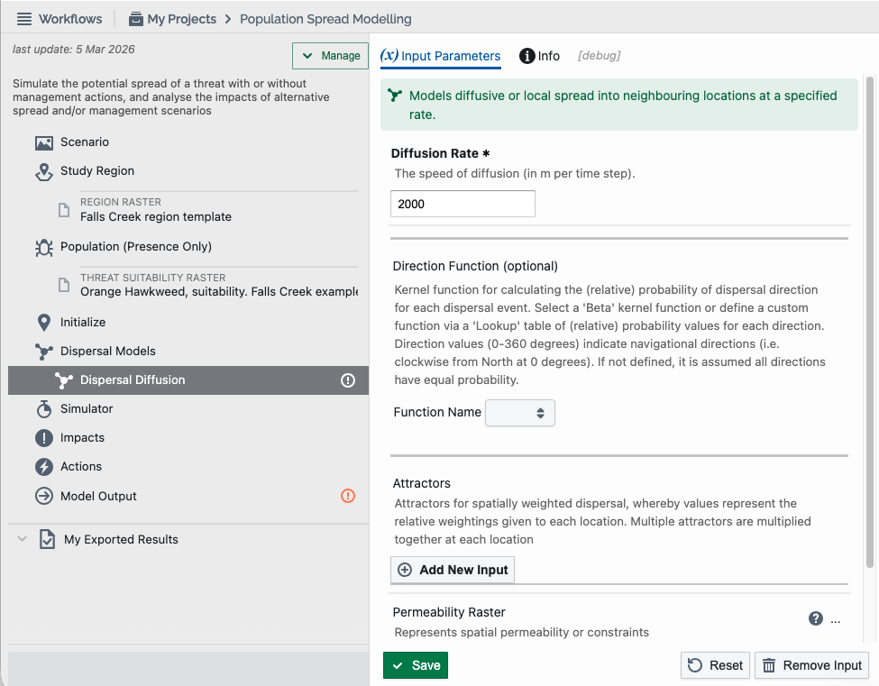
When users select Dispersal Diffusion, a new sub step appears in the tree prompting users to specify required and optional fields (see screenshot below). Dispersal diffusion models can only be used in grid models. Dispersal diffusion contains a range of required and optional fields that can be filled in. These include:
- Dispersal stages (Required for stage-structured populations only): See Kernel Dispersal (6.1) for description.
- Diffusion Rate (Required): The average rate of spread (in metres per time step).
- Direction Function (Optional): See Kernel Dispersal (6.1) for description.
- Direction orientation (Optional): See Kernel Dispersal (6.1) for description.
- Attractors (Optional): See Kernel Dispersal (6.1) for description.
- Permeability (Optional): See Kernel Dispersal (6.1) for description.
Select “Save” if enabled (note that data file selection may autosave your selections).
3. Dispersal Gravity
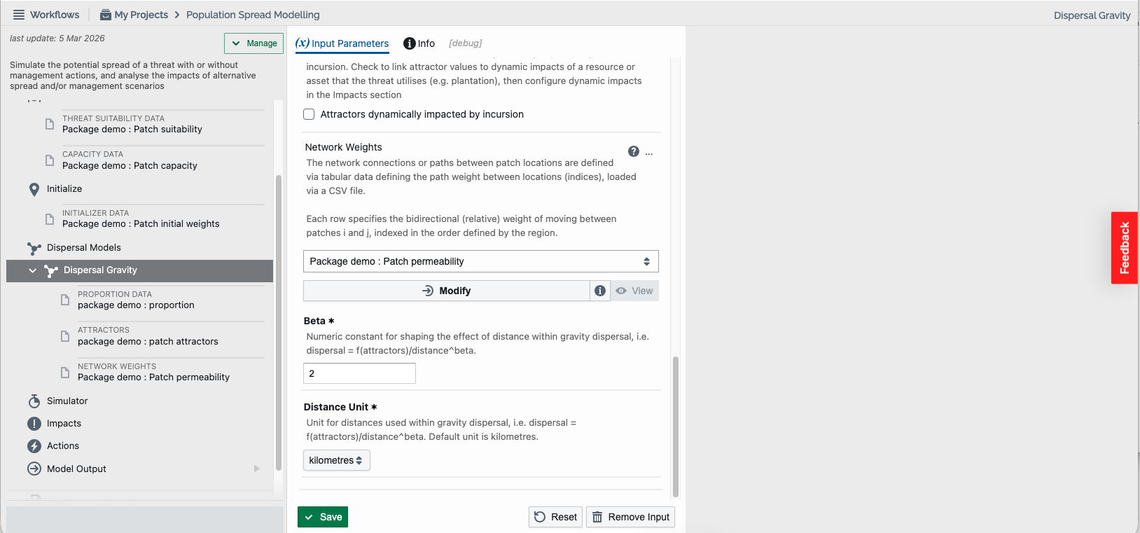
Network dispersal models commonly utilise a combination of spatially weighted attractors in combination with distances between nodes to determine the relative likelihood of movement between nodes. When selecting Dispersal Gravity a new sub step appears in the tree prompting users to specify required and optional fields. Dispersal gravity models can only be used in network models. Dispersal gravity contains a range of required and optional fields that can be filled in. These include:
- Dispersal stages (Required for stage-structured populations only): See Kernel Dispersal (6.1) for description.
- Proportion (Required for unstructured or stage-structured populations): See Kernel Dispersal for description.
- Events (Required for presence-only models; Optional for unstructured or stage-structured populations): See Kernel Dispersal (6.1) for description.
- Direction function (Optional): See Kernel Dispersal (6.1) for description.
- Direction orientation (Optional): See Kernel Dispersal (6.1) for description.
- Attractors (Required): See Kernel Dispersal (6.1) for description.
- Network weights (Optional): See Kernel Dispersal for description
- Beta (Required): A numeric constant for shaping the effect of distance within gravity dispersal, where dispersal = f(attractors)/distance^beta.
- Distance Unit (Required): Unit for distances used within gravity dispersal, i.e. dispersal = f(attractors)/distance^beta. The units selected should be the same for which beta is defined. Default unit is kilometres.
Select “Save” if enabled (note that data file selection may autosave your selections).
4. Radial Diffusion
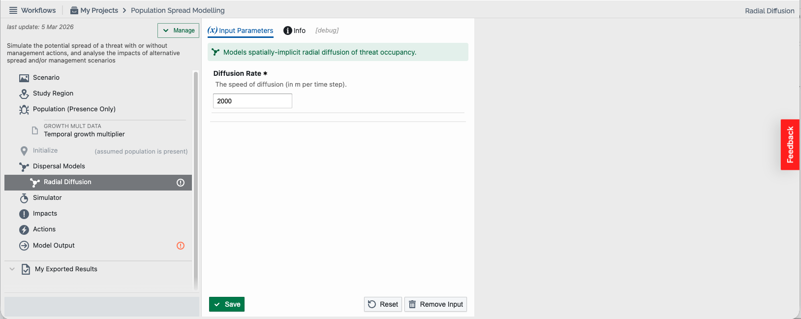
Radial diffusion is the most simplistic of spread functions that can be applied in a spatially implicit model with a presence-only population model. Radial diffusion spreads at a constant rate across an implicit homogeneous landscape with no constraints. When selecting Radial Diffusion a new sub step appears in the tree prompting users to specify a single parameter:
- Diffusion rate (Required): The average speed of diffusion (in metres per time step).
When you have finished, click the green “Save” button and you can move to the “Simulator” step in the tree.
5. Area Spread
Area spread is another simple dispersal function for spatially implicit models with unstructured or stage-structured population models. It contains no parameters, as it makes the explicit assumption that area of infestation increases proportionally with population size, which may be capacity limited.
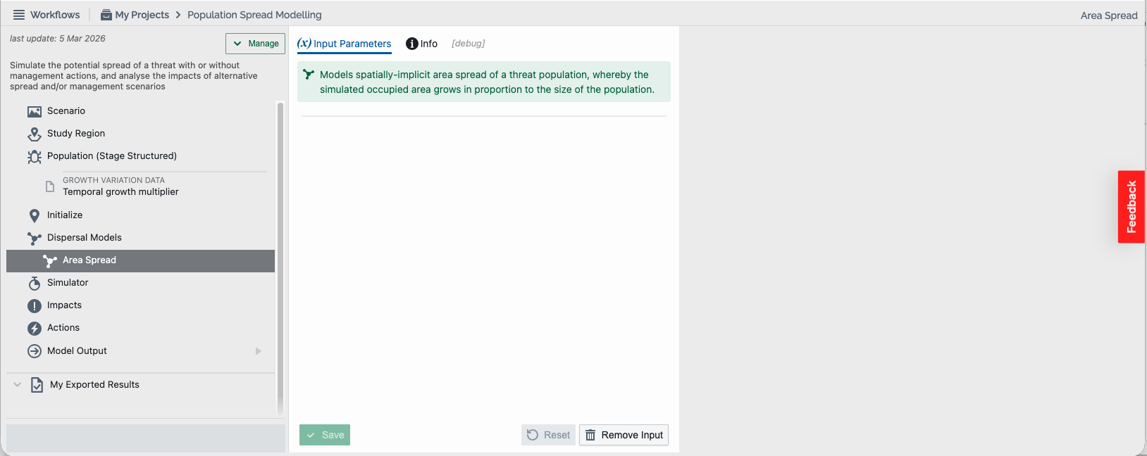
When you have finished, you can move to the “Simulator” step in the tree.
6. Reaction-Diffusion
Reaction-diffusion can be applied in spatially implicit models with unstructured or stage-structured population models. A reaction-diffusion dispersal model is a mathematical framework that describes the spatial and temporal spread of a population by combining two key processes: reaction (population growth) and diffusion (spatial spread). Within this function a single parameter must be specified (with other parameters specified in the Population and Study Region sections).
- Diffusion Rate (Required): The average rate of spread (in metres per time step)
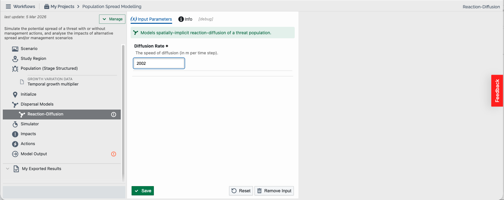
When you have finished, click the green “Save” button and you can move to the “Simulator” step in the tree.
Step 7. Configure the simulator
The Simulator allows users to set the overall parameters for the simulation including the number of time steps, their duration (including the time unit) and the number of simulations to be run (see screenshot below). Configure simulation via the following parameters:
- Time steps (Required): The number of discrete time steps to simulate.
- Step duration (Required): The duration of each discrete simulation time step along with its time unit (years, months, weeks, or days). The default step duration is 1 year. Configure other durations numerically with the appropriate unit (e.g. 3 months). This parameter allows users to specify the duration of a step that aligns with the biology of a species (e.g. generation times).
- Collation steps (Required): The interval in time steps for collating (spatial) results. The default is 1, whereby results are collated at every time step. Setting collation steps to a value greater than one avoids producing excessive spatial results (e.g. raster files) when many time steps are being simulated and the spatial distribution of the threat at every simulated time step is not essential.
- Replicates (Required): The number of repeated simulations to be run (range: 1 to 10,000). Note that replicate simulations results are collated as summary statistics (means and standard deviations) across simulations. Default is 1. It is important to note that threat dispersal is stochastically generated at each time step on (relative) probabilities (based on distance, direction, attraction, and/or permeability as per configured dispersal models), so results will change from one simulation to the next. Multiple simulations allow the user to obtain an overview of patterns (means and standard deviations) of possible dispersal (typically 1,000+ times when dispersal functions have probability distributions with wide or long tails).
- Combine Stages (Optional for stage-structured populations only): Select one or more checkboxes to combine (sum) specified stages within the results of a stage-based population model. If none are selected, the results are maintained for each stage.
TIP: Setting a high number of time steps and replicates can result in a long running simulation. Try conservative values initially until you are happy with your parameters.
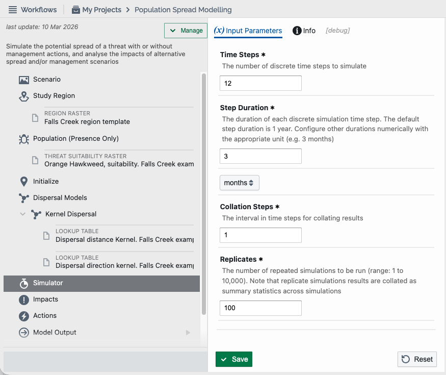
When you are ready click Save and move to the optional “Impacts” and/or “Actions” steps or proceed to the “Model Output” step to complete the experiment.
Step 8. Specify impacts (optional)
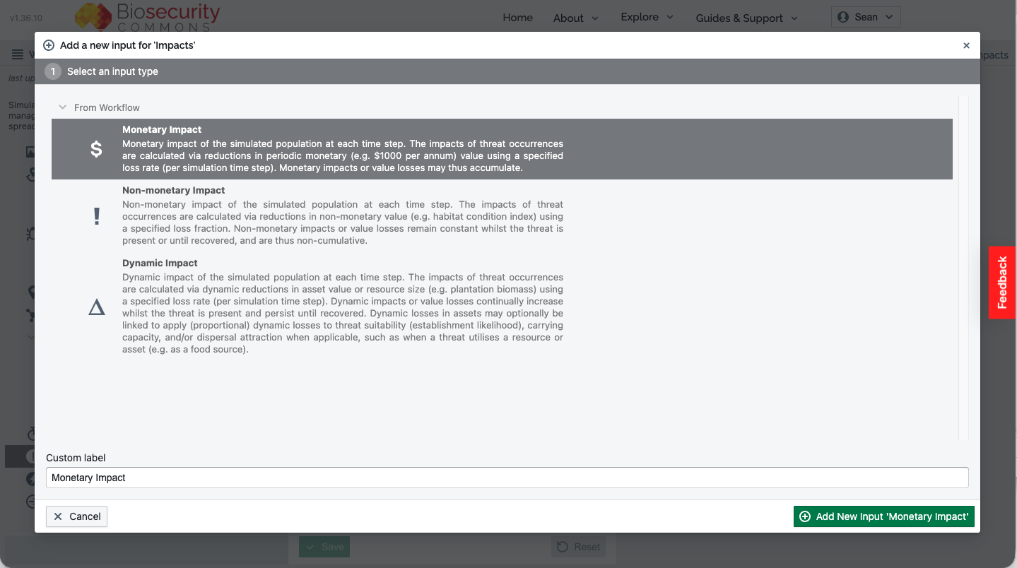
The impacts of the simulated threat may be calculated at each time step. Impacts may be specified as monetary loss in asset value (e.g. annual crops), non-monetary loss in quantified environmental or social features (e.g. species richness), or dynamic (accumulating) loss in an asset (e.g. plantation biomass). The three impact types are further described as follows:
- Monetary Impact: The impacts of threat occurrences are calculated via reductions in periodic monetary (e.g. $1000 per annum) value using a specified loss rate (per simulation time step). Monetary impacts or value losses may thus accumulate. Asset value may be discounted (% per annum/time step) to account for inflation. The recovery of assets may be delayed for an appropriate time-period, whereby impacts continue to be recorded after a simulated threat becomes absent.
- Non-monetary Impact: The impacts of threat occurrences are calculated via reductions in non-monetary value (e.g. habitat condition index) using a specified loss fraction. Non-monetary impacts or value losses remain constant whilst the threat is present or until recovered and are thus non-cumulative. The recovery of non-monetary assets may be delayed for an appropriate time-period, whereby impacts continue to be recorded after a simulated threat becomes absent.
- Dynamic Impact: The impacts of threat occurrences are calculated via dynamic reductions in asset value or resource size (e.g. plantation biomass) using a specified loss rate (per simulation time step). Dynamic impacts or value losses continually increase whilst the threat is present and persist until recovered. The recovery of assets may be delayed for an appropriate time-period, whereby impacts continue to be recorded after a simulated threat becomes absent. Dynamic losses in assets may optionally be linked to apply (proportional) dynamic losses to threat suitability (establishment likelihood), carrying capacity, and/or dispersal attraction when applicable, such as when a threat utilises a resource or asset (e.g. as a food source).
To add an impact, select “Add New Input” in the Impacts section of the tree:
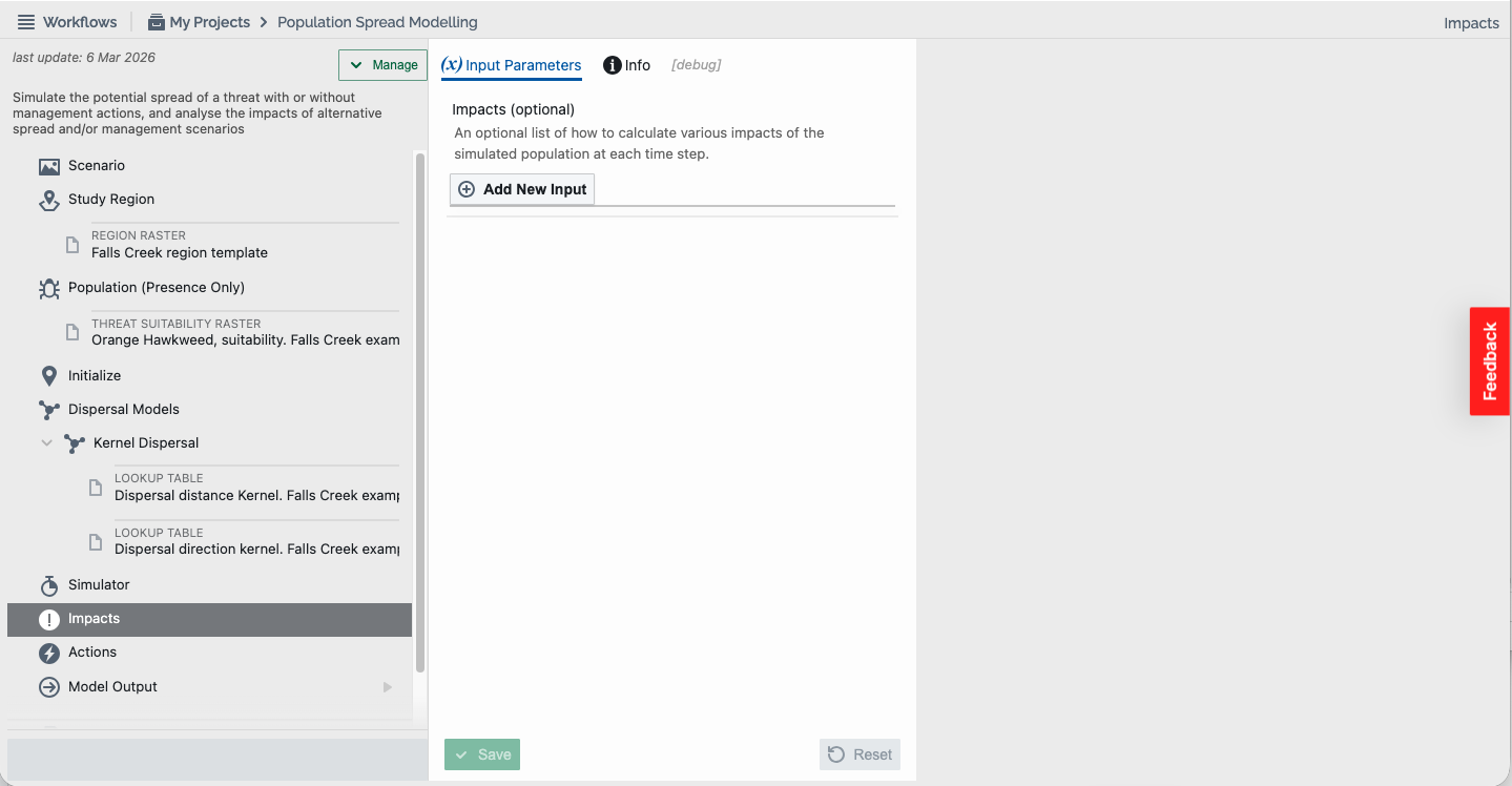
Then select the appropriate impact type for the threat scenario. When applicable, multiple impacts can be specified by the user (each added separately).
1. Monetary Impact
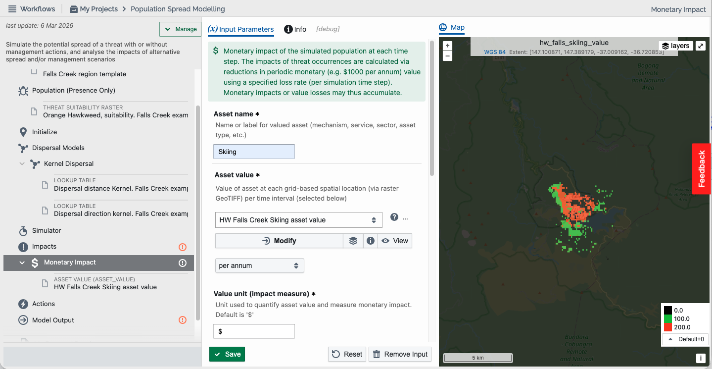
When users select Monetary Impact, a new sub step appears in the tree and multiple modification options will become available (see screenshot below). Monetary impact contains a range of required and optional fields that can be filled in or selected. These include:
- Asset name (Required): Name or label for valued asset (mechanism, service, sector, asset type, etc.).
- Asset value (Required): Value of the asset at each location (grid or network models) per annum or simulation time step (as per interval selected), or value per unit area (selected for spatially implicitmodels). Defined dependent on the study region model type selected in Step 3:
- Grid model – a raster grid (GeoTIFF)
- Network model – a CSV file having aligned ‘lon’, ‘lat’, and ‘value’ columns
- Spatially implicit model – a single value per unit area, which is selected as either ‘per metres squared’, ‘per kilometres squared’, or ‘across maximum area’ (when defined in the “Region” section)
- Value unit (Required): The unit of value or impact measure of the asset. Default is ‘$’ for monetary impacts.
- Impact type (Required for unstructured and stage-structured populations): Impacts may be calculated based on threat presence or density at each location. Select 'presence-based' (default) to simply apply the asset value loss (specified below) when the threat is present. Alternatively, select 'density-based' to scale the asset value loss (proportionally) via threat density (i.e. population size as a fraction of carrying capacity). Carrying capacity must be specified in the “Population” section for ‘density-based’ impacts, otherwise the impact type field will be absent, and the model will be configured with ‘presence-only’ impacts.
- Loss rate (Required): Loss of asset value per simulation time step when simulated incursion is present or until value is recovered (e.g. 0.2 for 20% loss per time step).
- Impact stages (Required for stage-structured populations only): Indicate which life-stages/ages contribute to impact. A checkbox will appear for each stage/age (i.e. column) specified in the growth matrix for users to select. If none are selected, all stages are assumed to be applicable.
- Discount rate (Optional): Discount rate per annum or simulation time step (as per interval selected) for the impacted asset values to estimate future values that account for inflation. Typically, the discounting uses market interest rates. Discounted impacts are calculated by dividing the value losses by
(1 + discount_rate)^time_int for simulated time intervals using the selected interval. E.g. set to 0.05 for a 5% per annum discount rate. - Asset recovery delay (Optional): Delay time in years or simulation time steps (as per selected) for assets to recover after local invasive species removal or extirpation. Impacts continue to be calculated as if the incursion were locally present for the recovery duration. Default is none, whereby calculated impacts become zero when an invasive species becomes locally absent.
Select “Save” if enabled (note that data file selection may autosave your selections).
2. Non-monetary Impact
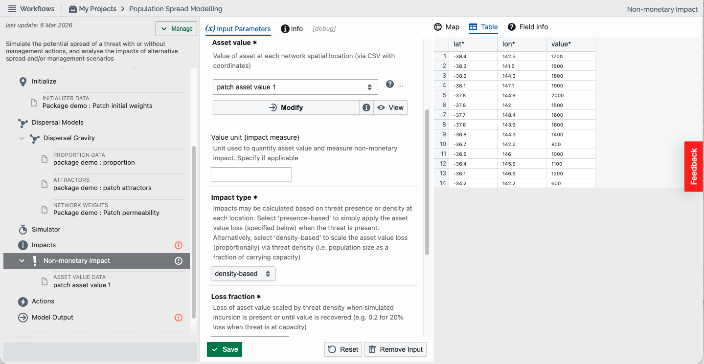
When users select Non-monetary Impact, a new sub step appears in the tree and multiple modification options will become available (see screenshot below). Non-monetary impact contains a range of required and optional fields that can be filled in or selected. These include:
- Asset name (Required): Name or label for valued asset (mechanism, service, sector, asset type, etc.).
- Asset value (Required): Value of the asset at each location (grid or network models) per annum or simulation time step (as per interval selected), or value per unit area (selected for spatially implicitmodels). Defined dependent on the study region model type selected in Step 3:
- Grid model – a raster grid (GeoTIFF)
- Network model – a CSV file having aligned ‘lon’, ‘lat’, and ‘value’ columns
- Spatially implicit model – a single value per unit area, which is selected as either ‘per metres squared’, ‘per kilometres squared’, or ‘across maximum area’ (when defined in the “Region” section)
- Value unit (Optional): The unit of value or impact measure of the asset.
- Impact type (Required for unstructured and stage-structured populations): Impacts may be calculated based on threat presence or density at each location. Select 'presence-based' (default) to simply apply the asset value loss (specified below) when the threat is present. Alternatively, select 'density-based' to scale the asset value loss (proportionally) via threat density (i.e. population size as a fraction of carrying capacity). Carrying capacity must be specified in the “Population” section for ‘density-based’ impacts, otherwise the impact type field will be absent, and the model will be configured with ‘presence-only’ impacts.
- Loss fraction (Required): Loss of asset value when simulated incursion is present or until value is recovered (e.g. 0.2 for 20% loss).
- Impact stages (Required for stage-structured populations only): Indicate which life-stages/ages contribute to impact. A checkbox will appear for each stage/age (i.e. column) specified in the growth matrix for users to select. If none are selected, all stages are assumed to be applicable.
- Asset recovery delay (Optional): Delay time in years or simulation time steps (as per selected) for assets to recover after local invasive species removal or extirpation. Impacts continue to be calculated as if the incursion were locally present for the recovery duration. Default is none, whereby calculated impacts become zero when an invasive species becomes locally absent.
Select “Save” if enabled (note that data file selection may autosave your selections).
3. Dynamic Impact
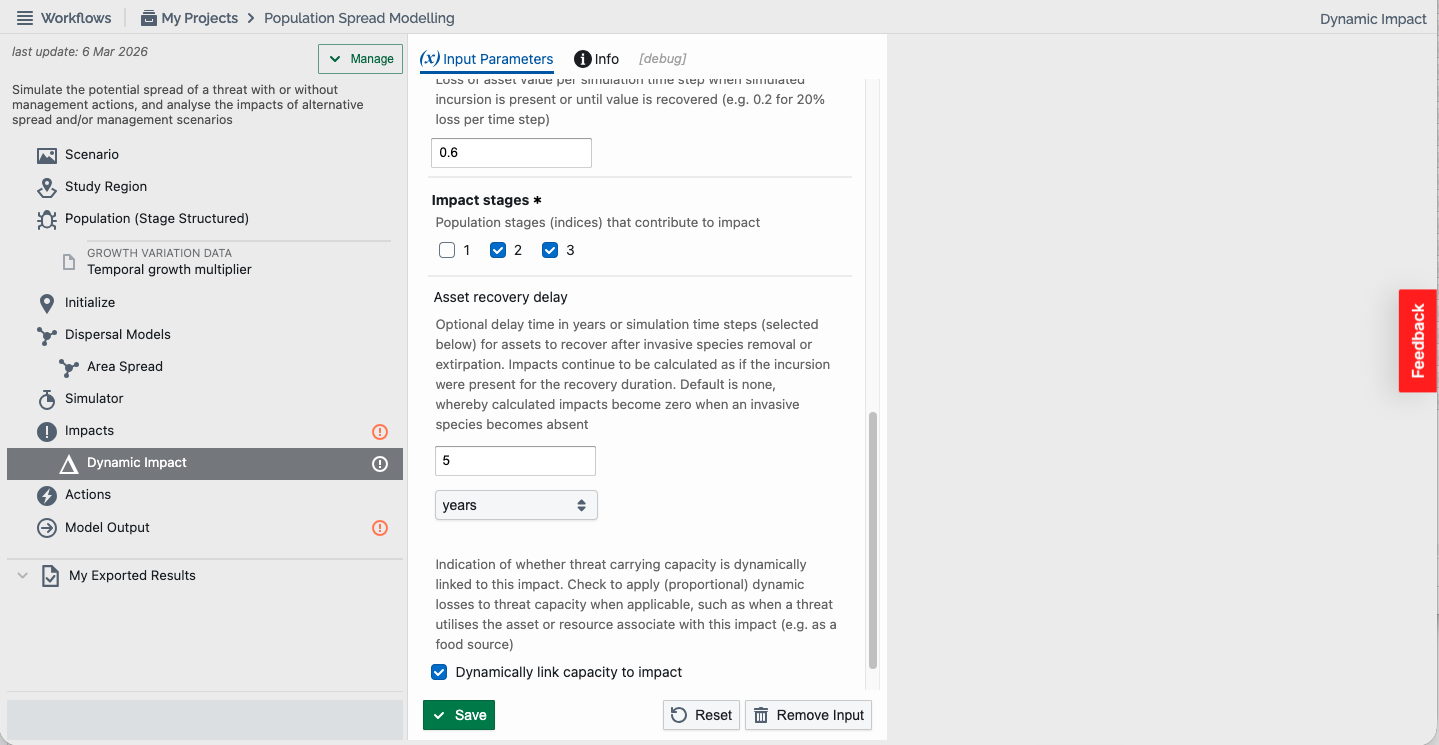
When users select Dynamic Impact, a new sub step appears in the tree and multiple modification options will become available (see screenshot below). Dynamic impact contains a range of required and optional fields that can be filled in or selected. These include:
- Asset name (Required): Name or label for valued asset (mechanism, service, sector, asset type, etc.).
- Asset value (Required): Value of the asset at each location (grid or network models) per annum or simulation time step (as per interval selected), or value per unit area (selected for spatially implicitmodels). Defined dependent on the study region model type selected in Step 3:
- Grid model – a raster grid (GeoTIFF)
- Network model – a CSV file having aligned ‘lon’, ‘lat’, and ‘value’ columns
- Spatially implicit model – a single value per unit area, which is selected as either ‘per metres squared’, ‘per kilometres squared’, or ‘across maximum area’ (when defined in the “Region” section)
- Value unit (Optional): The unit of value or impact measure of the asset.
- Loss fraction (Required): Loss of asset value when simulated incursion is present or until value is recovered (e.g. 0.2 for 20% loss).
- Impact stages (Required for stage-structured populations only): Indicate which life-stages/ages contribute to impact. A checkbox will appear for each stage/age (i.e. column) specified in the growth matrix for users to select. If none are selected, all stages are assumed to be applicable.
- Asset recovery delay (Optional): Delay time in years or simulation time steps (as per selected) for assets to recover after local invasive species removal or extirpation. Impacts continue to be calculated as if the incursion were locally present for the recovery duration. Default is none, whereby calculated impacts become zero when an invasive species becomes locally absent.
- Dynamically link suitability to impact (Optional for grid and network models only): Indication of whether threat suitability (likelihood of establishment) is dynamically linked to this impact. Check to apply (proportional) dynamic losses to threat suitability when applicable, such as when a threat utilises the asset or resource associate with this impact (e.g. as a food source). Only available when suitability is provided and the corresponding checkbox is checked in the “Population” section.
- Dynamically link capacity to impact (Optional for unstructured and stage-structured populations only): Indication of whether carrying capacity is dynamically linked to this impact. Check to apply (proportional) dynamic losses to threat capacity when applicable, such as when a threat utilises the asset or resource associate with this impact (e.g. as a food source). Only available when carrying capacity is provided and the corresponding checkbox is checked in the “Population” section.
- Dynamically link suitability to impact (Optional for unstructured and stage-structured populations only): Indication of whether dispersal attractors are dynamically linked to this impact. Check to apply (proportional) dynamic losses to threat dispersal destination attraction when applicable, such as when a threat utilises the asset or resource associate with this impact (e.g. as a food source). Only available when dispersal attractor(s) is provided and the corresponding checkbox is checked in the “Dispersal Models” section.
Select “Save” if enabled (note that data file selection may autosave your selections).
Step 9. Specify actions (optional)
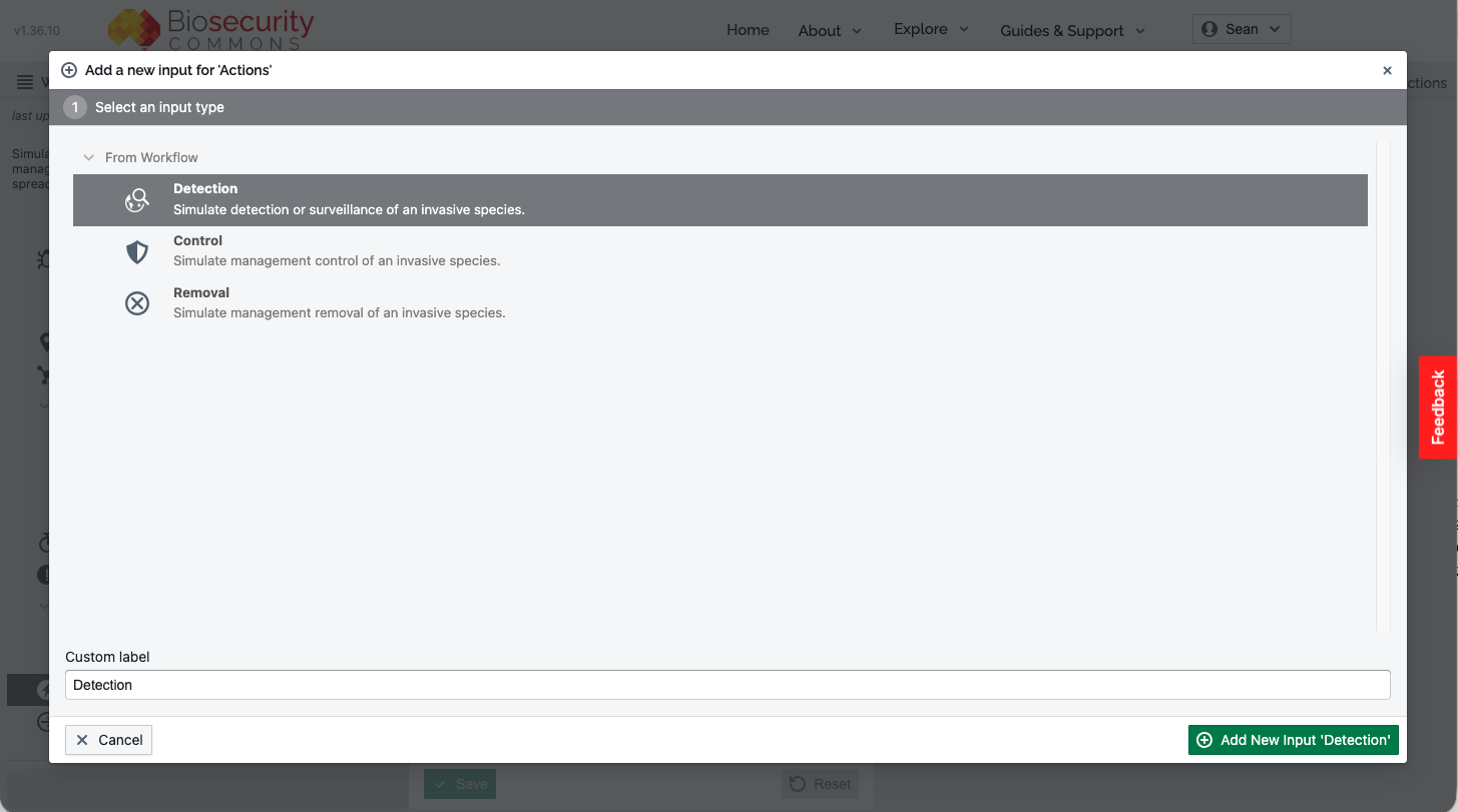
Management actions may be applied within the population spread model simulations. Actions include the application of surveillance designs for threat detection, threat control actions, and threat removal. These action types are further described as follows:
- Detection: Simulate detection or surveillance of an invasive threat utilising the sensitivity (detection probability) of a scheduled surveillance system (design), along with surveillance costs.
- Control: Simulate the application of management control of an invasive threat, including scheduled “search & destroy” (combined detection & removal), growth, spread, and establishment controls, along with their application costs.
- Removal: Simulate the removal of an invasive threat, including scheduled management and their costs, as well as likely removal via other public initiatives.
To add an action, select “Add New Input” in the Actions section of the tree:
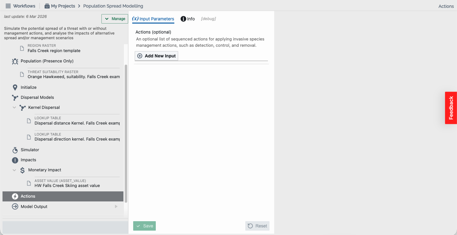
Then select the appropriate action type for the threat scenario. When applicable, multiple actions can be specified by the user (each added separately).
1. Detection
When users select Detection, a new sub step appears in the tree and multiple modification options will become available (see screenshot below). Detection actions contain a range of required and optional fields that can be filled in or selected. These include:
- Detection probability (Required): Probability of detection (surveillance sensitivity) at each location (grid or network models), or single value (spatially implicitmodels). Defined dependent on the study region model type selected in Step 3:
- Grid model – a raster grid (GeoTIFF)
- Network model – a CSV file having aligned ‘lon’, ‘lat’, and ‘sensitivity’ columns
- Spatially implicit model – a single value
The detection probability or sensitivity values may be added using the output results from a Surveillance Design workflow by selecting “Choose from My Results” when adding the input, then navigating to the exported result for the appropriate Surveillance Design project (note: must be exported from that project).
- Sensitivity type (Required for unstructured and stage-structured populations): Select how detection probability (sensitivity) is specified:
- Individual level – The sensitivity is specified at the individual level, whereby sensitivity values denote the probability of detection for each (detectable) invasive individual.
- Population size (threshold) level – The sensitivity is specified based on the size of the population, whereby sensitivity values denote the probability of detecting (local) populations having at least at certain size (of detectable individuals), specified via a threshold value (below). The probability of detecting (local) population sizes below the threshold value is reduced proportionally (i.e. scaled by size/threshold).
- Presence/absence level – The sensitivity is specified at the presence/absence level, whereby sensitivity values denote the probability of detecting any (local) presence of (detectable individuals within) the invasive species population (equivalent to threshold = 1).
- Sensitivity threshold (Required when the sensitivity type is specified at the population size level): The threshold (minimum) population size (of detectable individuals) for (locally) applying the specified detection probability (sensitivity) values. The probability of detection for (local) population sizes below the threshold value is reduced proportionally (i.e. scaled by size/threshold).
- Stages (Required for stage-structured populations only): Indicate which life-stages/ages are detected. A checkbox will appear for each stage/age (i.e. column) specified in the growth matrix for users to select. If none are selected, all stages are assumed to be applicable.
- Surveillance cost (Optional): Optional cost of each application of surveillance (whether successful or not) at each location (grid or network models), or across the entire area (spatially implicitmodels). Specify cost via selection:
- Single value (all models) – to configure a uniform value across the region
- Across locations (grid & network models) – to configure values at each location, defined dependent on the study region model type selected in Step 3:
- Grid model – a raster grid (GeoTIFF)
- Network model – a CSV file having aligned ‘lon’, ‘lat’, and ‘surv_cost’ columns
- Cost unit (Optional): Unit used to quantify surveillance cost. Default is '$'.
- Schedule (Required): Select the appropriate simulation time steps in which to apply surveillance. “Select All” and “None” buttons are available for convenience.
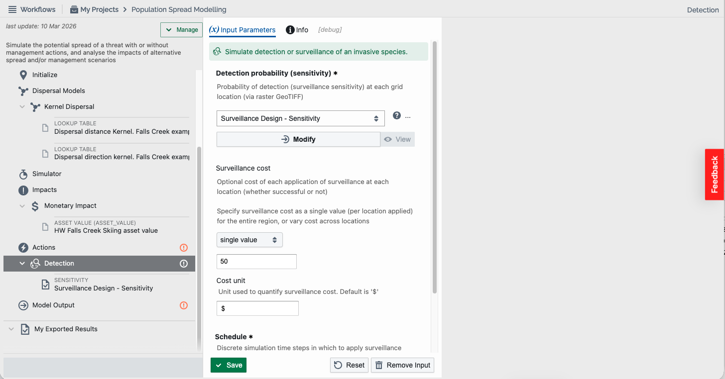
Select “Save” if enabled (note that data file selection may autosave your selections).
2. Control
When users select Control, a new sub step appears in the tree and multiple modification options will become available (see screenshot below). Control actions contain a range of required and optional fields that can be filled in or selected, which vary depending on the desired control type:
- Control type (Required): Select the type of control to be applied to the invasive species from:
- Search and destroy (all models) – Combined surveillance and removal. Useful for scenarios when the surveillance method used also involves removing detected threats (e.g. manual survey control, lethal trapping).
- Growth control (unstructured and stage-structured populations only) – Reduce or suppress threat growth. Useful to simulate scenarios that use treatments to reduce or suppress growth (e.g. chemical or biological agents).
- Spread control (grid and network models only) – Reduce or suppress threat spread events. Useful to simulate scenarios that place restrictions on threat spread (e.g. spread barriers, quarantine, transport restrictions).
- Establishment control (grid and network models only) – Reduce or suppress establishment of threat arrivals. Useful to simulate scenarios that inhibit the establishment of threats in new locations (e.g. chemical treatments or biological agents).
Depending on the control type the user selects, different options will become available. Next, users specify either:
2.1. Search and destroy type
- Control effectiveness (Required): Control effectiveness (probability of management success) at each location (grid or network models), or single value (spatially implicitmodels). Defined dependent on the study region model type selected in Step 3:
- Grid model – a raster grid (GeoTIFF)
- Network model – a CSV file having aligned ‘lon’, ‘lat’, and ‘manage_pr’ columns
- Spatially implicit model – a single value
The control effectiveness (management probability) values may be added using the output results from a Resource Allocation Design workflow by selecting “Choose from My Results” when adding the input, then navigating to the exported result for the appropriate Resource Allocation project (note: must be exported from that project).
- Control effectiveness type (Required for unstructured and stage-structured populations): Select how control effectiveness (management probability) is specified:
- Individual level – The effectiveness is specified at the individual level, whereby effectiveness values denote the probability of control success for each (controllable) invasive individual.
- Population level – The effectiveness is specified based on the entire (local) population, whereby effectiveness values denote the probability of controlling all (controllable) individuals within the (local) invasive population.
- Stages (Required for stage-structured populations only): Indicate which life-stages/ages to which control is applied. A checkbox will appear for each stage/age (i.e. column) specified in the growth matrix for users to select. If none are selected, all stages are assumed to be applicable.
- Control cost (Optional): Optional cost of each application of control (whether successful or not) at each location (grid or network models), or across the entire area (spatially implicitmodels). Specify cost via selecting:
- Single value (all models) – to configure a uniform value across the region
- Across locations (grid & network models) – to configure values at each location, defined dependent on the study region model type selected in Step 3:
- Grid model – a raster grid (GeoTIFF)
- Network model – a CSV file having aligned ‘lon’, ‘lat’, and ‘control_cost’ columns
- Cost unit (Optional): Unit used to quantify control cost. Default is '$'.
- Schedule (Required): Select the appropriate simulation time steps in which to apply control. “Select All” and “None” buttons are available for convenience.
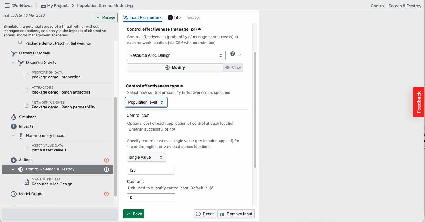
Select “Save” if enabled (note that data file selection may autosave your selections).
2.2. Growth control type
- Control multiplier (Required): Multiplier(s) (0-1) applied to growth rate (unstructured models) or stage/age transition rates (stage-structured models) to reduce or suppress overall growth of the threat when the threat is detected via surveillance actions if present. Specify multiplier via selection:
- Single value (all models) – to configure a uniform value across the region
- Across locations (grid & network models) – to configure values at each location, defined dependent on the study region model type selected in Step 3:
- Grid model – a raster grid (GeoTIFF)
- Network model – a CSV file having aligned ‘lon’, ‘lat’, and ‘control_mult’ columns
For stage-structured models, multipliers may be applied to reproduction, survival, or both, as well as to selected stages. These options (selected below) may be utilised together, for example, to control the seasonal survival rates of specified life stages.
- Existing control (Optional for grid & network models only): Optional existing, known, or scheduled control application locations. Defined dependent on the study region model type selected in Step 3:
- Grid model – a raster grid (GeoTIFF)
- Network model – a CSV file having aligned ‘lon’, ‘lat’, and ‘exist_control’ columns
- Control radius (Optional for grid & network models only): Optional radius (in metres) of control surroundings. The control is applied to all locations within the specified radius of each location where the threat has been detected (if surveillance actions are present). Default (none) indicates that control is only applied at detected locations.
- Apply control to (Required for stage-structured populations only): Growth control may be applied to (select):
- Reproduction – the number of early stage/age offspring or seeds produced
- Survival – the rate of survival for each stage/age
- Both – reproduction and survival (all stage matrix transition rates)
- Stages (Required for stage-structured populations only): Indicate which life-stages/ages to which control is applied. A checkbox will appear for each stage/age (i.e. column) specified in the growth matrix for users to select. If none are selected, all stages are assumed to be applicable.
- Control cost (Optional): Optional cost of each application of control (whether successful or not) at each location (grid or network models), or per specified area (spatially implicitmodels). Specify cost via selecting:
- Single value (all models) – to configure a uniform value:
- At every location cross the region (grid & network models)
- Per specified area (spatially implicitmodels), selected:
- Per metres squared (default)
- Per kilometres squared
- Across locations (grid & network models) – to configure values at each location, defined dependent on the study region model type selected in Step 3:
- Grid model – a raster grid (GeoTIFF)
- Network model – a CSV file having aligned ‘lon’, ‘lat’, and ‘control_cost’ columns
- Single value (all models) – to configure a uniform value:
- Cost unit (Optional): Unit used to quantify control cost. Default is '$'.
- Schedule (Required): Select the appropriate simulation time steps in which to apply control. “Select All” and “None” buttons are available for convenience.
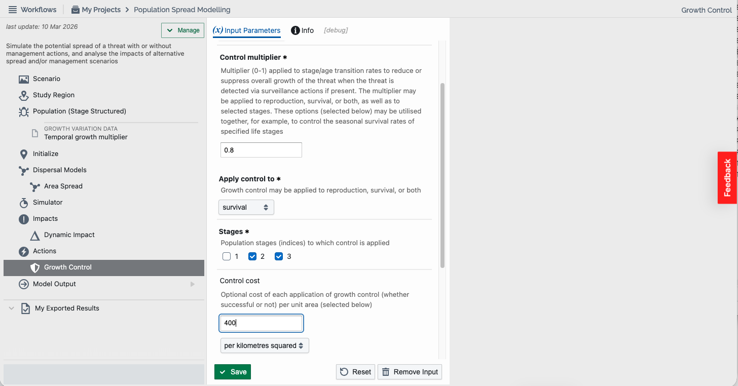
Select “Save” if enabled (note that data file selection may autosave your selections).
2.3. Spread control type
- Control multiplier (Required): Multiplier(s) (0-1) applied to the number of dispersal events to reduce or suppress spread of the threat from each grid or network model location (and optionally surroundings) where the threat is detected (if surveillance actions are present), as well as existing, known, or scheduled control treatment locations (optionally specified below) occupied by the threat. Specify multiplier via selection:
- Single value – to configure a uniform value across the region
- Across locations – to configure values at each location, defined dependent on the study region model type selected in Step 3:
- Grid model – a raster grid (GeoTIFF)
- Network model – a CSV file having aligned ‘lon’, ‘lat’, and ‘control_mult’ columns
For stage-structured models, multipliers may be applied to reproduction, survival, or both, as well as to selected stages. These options (selected below) may be utilised together, for example, to control the seasonal survival rates of specified life stages.
- Existing control (Optional for grid & network models only): Optional existing, known, or scheduled control application locations. Defined dependent on the study region model type selected in Step 3:
- Grid model – a raster grid (GeoTIFF)
- Network model – a CSV file having aligned ‘lon’, ‘lat’, and ‘exist_control’ columns
- Control radius (Optional for grid & network models only): Optional radius (in metres) of control surroundings. The control is applied to all locations within the specified radius of each location where the threat has been detected (if surveillance actions are present). Default (none) indicates that control is only applied at detected locations.
- Stages (Required for stage-structured populations only): Indicate which life-stages/ages to which control is applied. A checkbox will appear for each stage/age (i.e. column) specified in the growth matrix for users to select. If none are selected, all stages are assumed to be applicable.
- Control cost (Optional): Optional cost of each application of control (whether successful or not) at each location (grid or network models). Specify cost via selecting:
- Single value – to configure a uniform value across the region
- Across locations – to configure values at each location, defined dependent on the study region model type selected in Step 3:
- Grid model – a raster grid (GeoTIFF)
- Network model – a CSV file having aligned ‘lon’, ‘lat’, and ‘control_cost’ columns
- Cost unit (Optional): Unit used to quantify control cost. Default is '$'.
- Schedule (Required): Select the appropriate simulation time steps in which to apply control. “Select All” and “None” buttons are available for convenience.
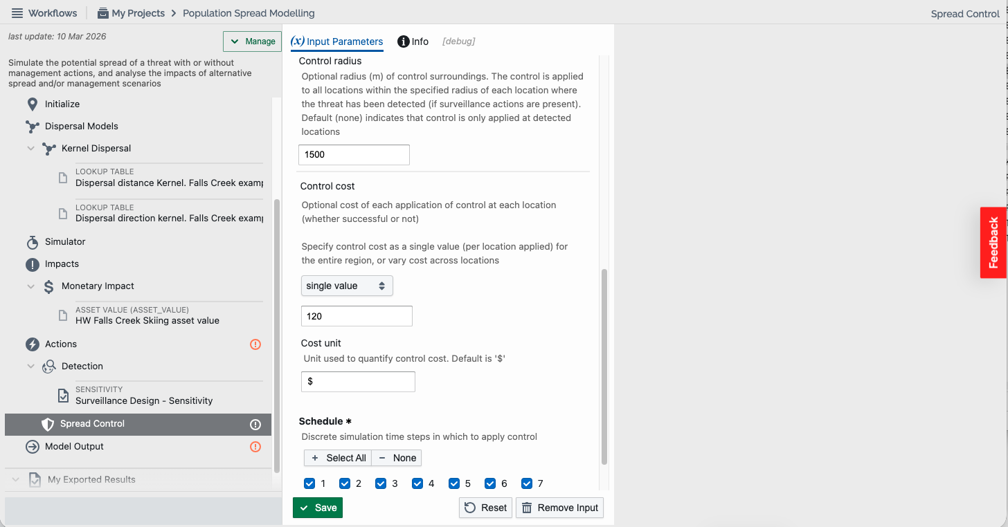
Select “Save” if enabled (note that data file selection may autosave your selections).
2.4. Establishment control type
- Control multiplier (Required): Multiplier(s) (0-1) applied to the establishment probability to reduce or suppress establishment of threat arrivals in each grid or network model location (and optionally surroundings) where the threat is detected (if surveillance actions are present), as well as existing, known, or scheduled control treatment locations (optionally specified below) occupied by the threat. Specify multiplier via selection:
- Single value – to configure a uniform value across the region
- Across locations – to configure values at each location, defined dependent on the study region model type selected in Step 3:
- Grid model – a raster grid (GeoTIFF)
- Network model – a CSV file having aligned ‘lon’, ‘lat’, and ‘control_mult’ columns
For stage-structured models, multipliers may be applied to reproduction, survival, or both, as well as to selected stages. These options (selected below) may be utilised together, for example, to control the seasonal survival rates of specified life stages.
- Existing control (Optional for grid & network models only): Optional existing, known, or scheduled control application locations. Defined dependent on the study region model type selected in Step 3:
- Grid model – a raster grid (GeoTIFF)
- Network model – a CSV file having aligned ‘lon’, ‘lat’, and ‘exist_control’ columns
- Control radius (Optional for grid & network models only): Optional radius (in metres) of control surroundings. The control is applied to all locations within the specified radius of each location where the threat has been detected (if surveillance actions are present). Default (none) indicates that control is only applied at detected locations.
- Stages (Required for stage-structured populations only): Indicate which life-stages/ages to which control is applied. A checkbox will appear for each stage/age (i.e. column) specified in the growth matrix for users to select. If none are selected, all stages are assumed to be applicable.
- Control cost (Optional): Optional cost of each application of control (whether successful or not) at each location (grid or network models). Specify cost via selecting:
- Single value – to configure a uniform value across the region
- Across locations – to configure values at each location, defined dependent on the study region model type selected in Step 3:
- Grid model – a raster grid (GeoTIFF)
- Network model – a CSV file having aligned ‘lon’, ‘lat’, and ‘control_cost’ columns
- Cost unit (Optional): Unit used to quantify control cost. Default is '$'.
- Schedule (Required): Select the appropriate simulation time steps in which to apply control. “Select All” and “None” buttons are available for convenience.
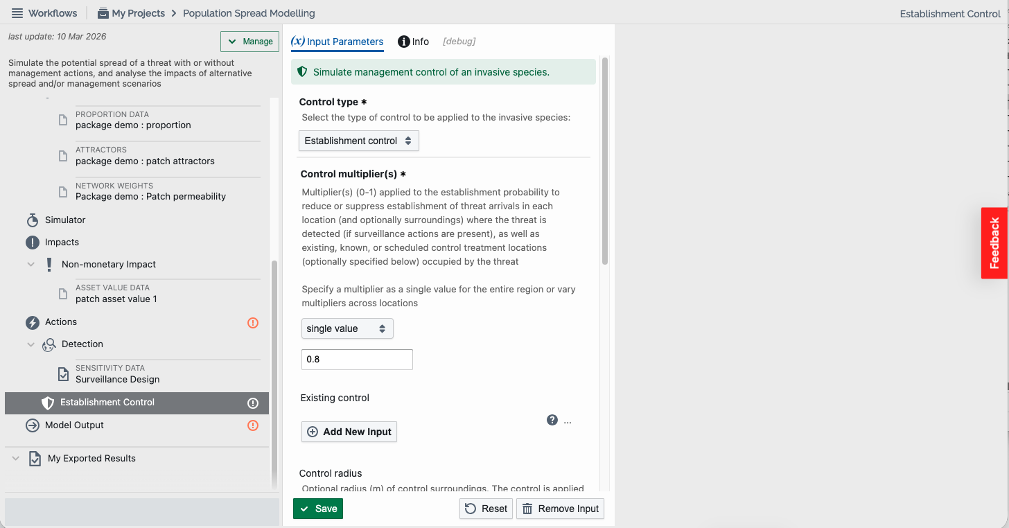
Select “Save” if enabled (note that data file selection may autosave your selections).
3. Removal
When users select Removal, a new sub step appears in the tree and multiple modification options will become available (see screenshot below). Removal actions contain a range of required and optional fields that can be filled in or selected. These include:
- Removal probability (Required): Probability of removal at each location (grid or network models), or single value (spatially implicitmodels). Specify probability via selection:
- Single value (all models) – to configure a uniform value across the region
- Across locations (grid & network models) – to configure values at each location, defined dependent on the study region model type selected in Step 3:
- Grid model – a raster grid (GeoTIFF)
- Network model – a CSV file having aligned ‘lon’, ‘lat’, and ‘removal_pr’ columns
- Removal probability type (Required for unstructured and stage-structured populations): Select how removal probability is specified:
- Individual level – The removal probability is specified at the individual level, whereby probability values denote the probability of removal success for each (removable) invasive individual.
- Population level – The removal probability is specified based on the entire (local) population, whereby probability values denote the probability of removing all (removable) individuals within the (local) invasive population.
- Always apply removal (Optional): Select to indicate that removal is always to applied to locations where invasive species are present (even when they are not detected by surveillance actions). When unselected (default) removal is dependent on detection when surveillance actions are present. Select when some removal is likely regardless of explicit management efforts (e.g. removal by the public or property owners).
- Only remove detected individuals (Optional for unstructured and stage-structured populations when detection is specified at the individual level): Select to indicate that removal is only applied to detected individuals (e.g. via traps). When unselected (default) removal is applied to all individuals at locations where the invasive species has been detected (e.g. via treatment).
- Removal radius (Optional for grid & network models only): Optional radius (in metres) of removal surroundings. Removal is applied to all locations within the specified radius of each location where the threat has been detected (if surveillance actions are present). Default (none) indicates that removal is only applied at detected locations.
- Stages (Required for stage-structured populations only): Indicate which life-stages/ages to which removal is applied. A checkbox will appear for each stage/age (i.e. column) specified in the growth matrix for users to select. If none are selected, all stages are assumed to be applicable.
- Removal cost (Optional): Optional cost of each application of removal (whether successful or not) at each location (grid or network models), or per specified area (spatially implicitmodels). Specify cost via selection:
- Single value (all models) – to configure a uniform value:
- At every location cross the region (grid & network models)
- Per specified area (spatially implicitmodels), selected:
- Per metres squared (default)
- Per kilometres squared
- Across locations (grid & network models) – to configure values at each location, defined dependent on the study region model type selected in Step 3:
- Grid model – a raster grid (GeoTIFF)
- Network model – a CSV file having aligned ‘lon’, ‘lat’, and ‘removal_cost’ columns
- Single value (all models) – to configure a uniform value:
- Cost unit (Optional): Unit used to quantify removal cost. Default is '$'.
- Schedule (Required): Select the appropriate simulation time steps in which to apply removal. “Select All” and “None” buttons are available for convenience.
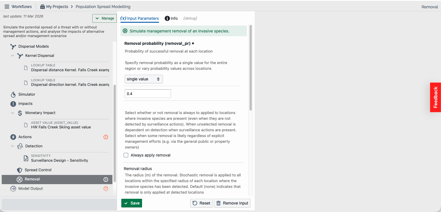
Select “Save” if enabled (note that data file selection may autosave your selections).
Step 10. Run the population spread model
Once the model branches and subbranches have been successfully configured (with no exclamation marks to indicate incomplete sections), you will be able to run your population spread model simulation. Select “Model Output” in the tree, then click the “Run” button in the bottom left-hand corner to run the workflow (see screenshot below).

The output page will be updated as the job progresses from “Created”, “Submitted”, and “Success”.
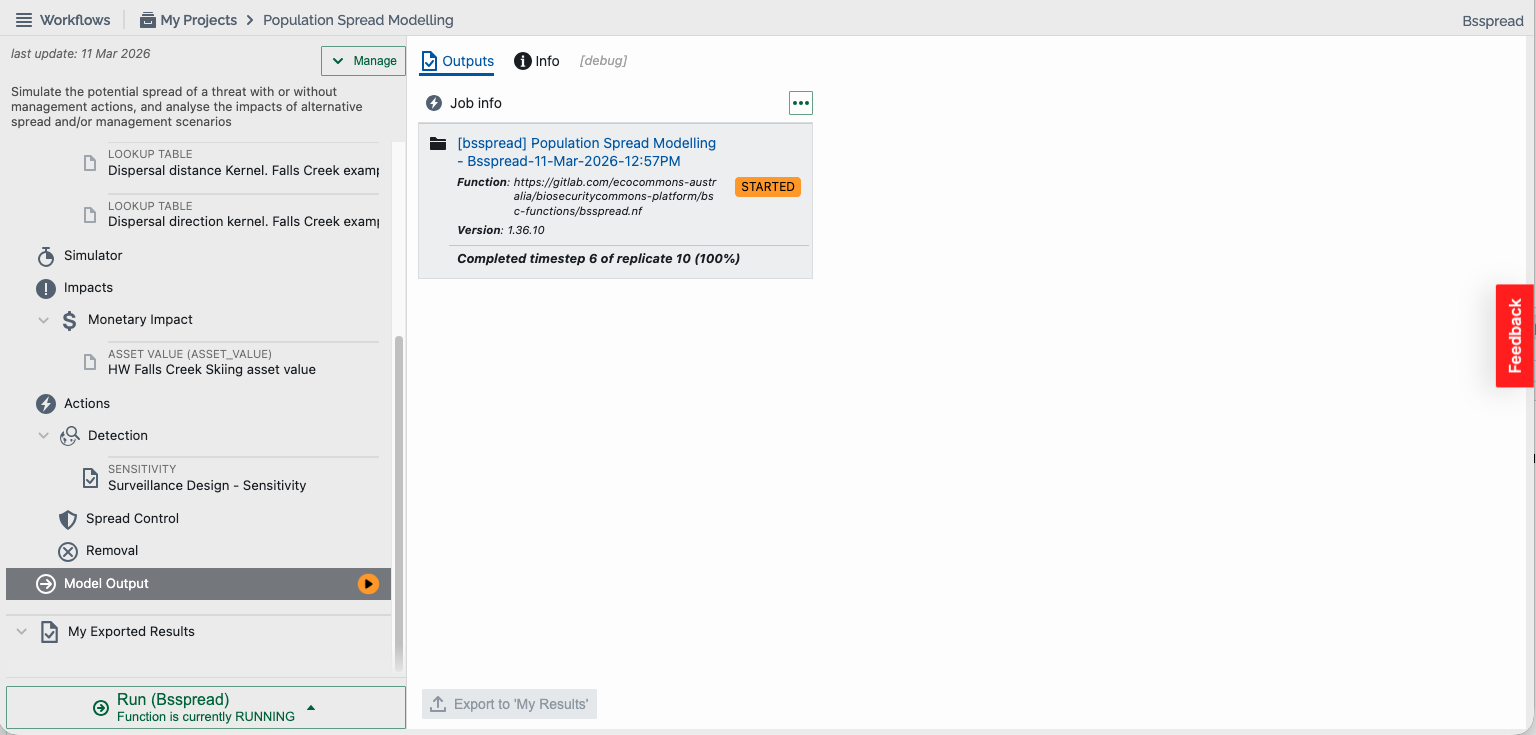
Once it has finished, a green tick will appear next to “Model Output”, and the user will be able to view and download the outputs (example screenshot below):
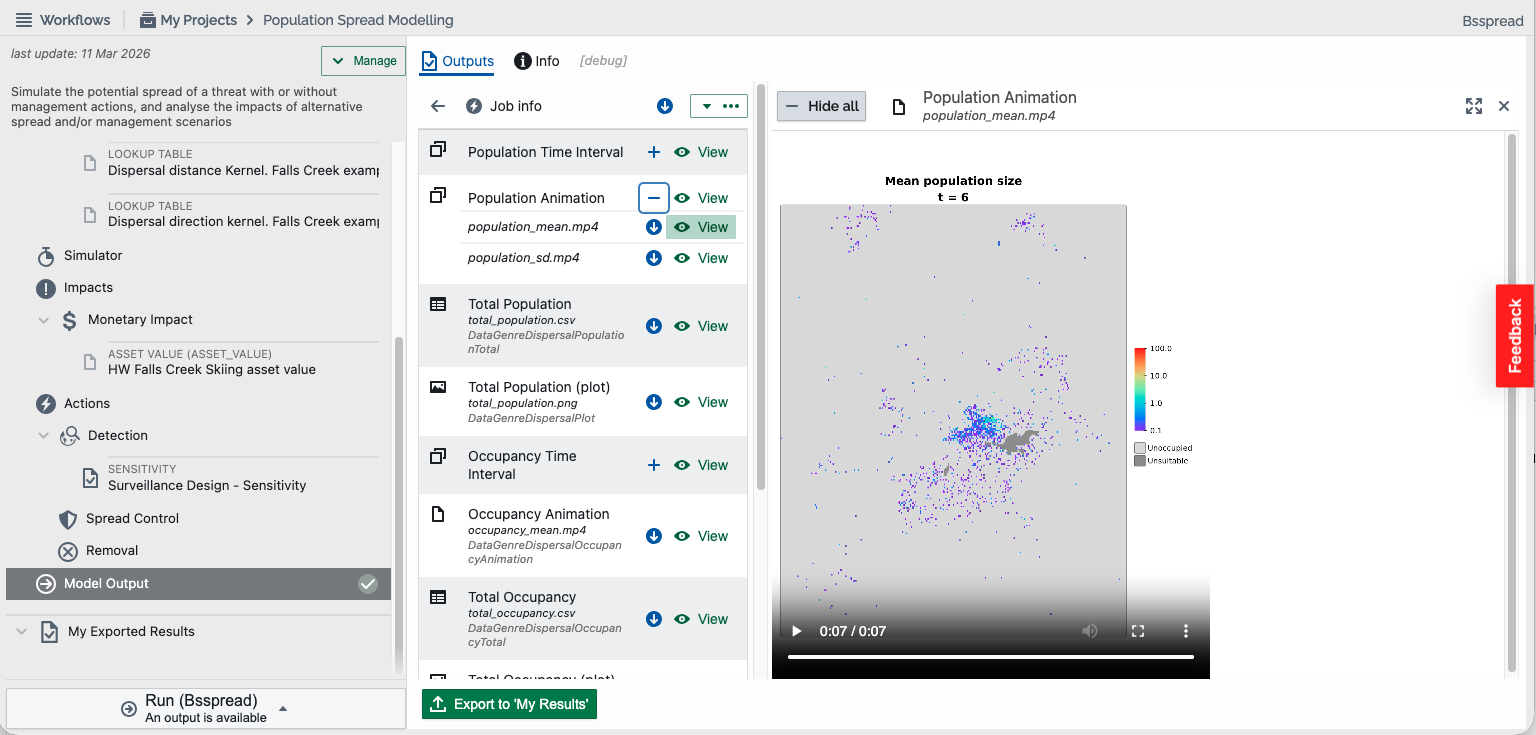
The outputs provided depend on the model region type (grid, network, or spatially implicit) and population model type (presence-only, unstructured, or stage-structured) selected, and the impacts (monetary, non-monetary, and/or dynamic) and actions (detection, control, and/or removal) optionally added by the user. Other simulation outputs, including platform workflow & job information, are also generated. The following is a summary of outputs for each model region type:
1. Grid model outputs
- Population Time Interval (unstructured models or stage-structured models with combined result stages): A drop-down list of raster (GeoTIFF) files. For single-replicate runs, the files will contain the number of individuals at each location for each collated time step. Multiple-replicate runs generate separate files for the mean & standard deviation of the number of individuals for each collated time step.
- Population Stage Time Interval (stage-structured models with separate result stages only): A drop-down list of raster (GeoTIFF) files containing the number of individuals (or multi-replicate mean & standard deviation) at each location for each population stage for each collated time step.
- Population Animation (unstructured or stage-structured models only): One or more grid-based animations of the simulated population number of individuals across the collated time steps. Animation (MP4) files are generated using the Population Time Interval or Population Stage Time Interval raster (GeoTIFF) files above, thus separate animations are generated for multi-replicate mean and standard deviations and/or stages when applicable.
- Total Population (unstructured or stage-structured models only): One or more tabular comma-separated values (CSV) files containing the total number of individuals (or multi-replicate mean & standard deviation) at each time step. These numbers are listed separately for each stage when applicable. The combination of separate stages and multiple replicates results in separate files being generated for each stage, else the separate stages or summary statistics (mean & SD) are placed in tabular rows.
- Total Population (plot) (unstructured or stage-structured models only): One or more graphic (PNG) files each containing a time-series plot of the total number of individuals (or multi-replicate mean +/- 2 standard deviations). For example:
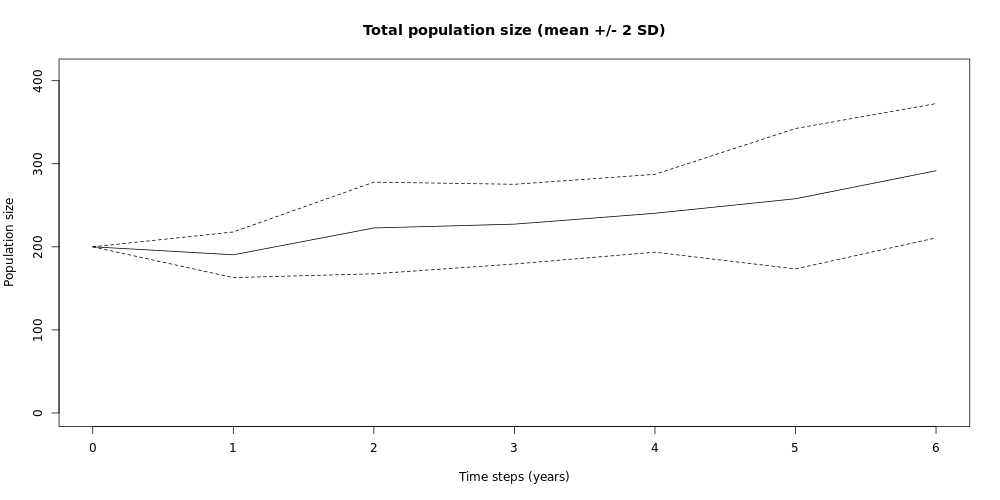 Multiple plot files are generated for each stage when applicable.
- Occupancy Time Interval (all population models): A drop-down list of raster (GeoTIFF) files. For single-replicate runs, the files will contain the threat occupancy (or binary presence/absence), or mean occupancy for multiple replicates, at each location for each collated time step.
- Occupancy Animation (all population models): A grid-based animation of the simulated threat occupancy or mean occupancy across the collated time steps. The animation (MP4) file is generated using the Occupancy Time Interval raster (GeoTIFF) files above.
- Total Occupancy (all population models): A tabular (CSV) file containing the total number of occupied locations (or multi-replicate mean & standard deviation) at each time step. The separate summary statistics (mean & SD) are placed in tabular rows when applicable.
- Total Occupancy (plot) (all population models): A graphic (PNG) file containing a time-series plot of the total number of occupied locations (or multi-replicate mean +/- 2 standard deviations).
- Total Area Occupied (all population models): A tabular (CSV) file containing the total area (in metres squared) occupied by the threat (or multi-replicate mean & standard deviation) at each time step. The separate summary statistics (mean & SD) are placed in tabular rows when applicable.
- Total Area Occupied (plot) (all population models): A graphic (PNG) file containing a time-series plot of the total area (in metres squared) occupied by the threat (or multi-replicate mean +/- 2 standard deviations).
- Impacts (optionally added): A drop-down list of raster (GeoTIFF) files. For single-replicate runs, the files will contain the calculated impacts at each location for each collated time step for each added impact. Multiple-replicate runs generate separate files for the mean & standard deviation of the impacts for each collated time step.
- Impacts Animation (optionally added): One or more grid-based animations of the simulated impacts across the collated time steps for each added impact. Animation (MP4) files are generated using the Impacts raster (GeoTIFF) files above, thus separate animations are generated for multi-replicate mean and standard deviations when applicable.
- Cumulative Impacts (optionally added): A drop-down list of raster (GeoTIFF) files. For single-replicate runs, the files will contain the calculated cumulative impacts (across time) at each location for each collated time step for each added impact. Multiple-replicate runs generate separate files for the mean & standard deviation of the cumulative impacts for each collated time step.
- Cumulative Impacts Animation (optionally added): One or more grid-based animations of the simulated cumulative impacts across the collated time steps for each added impact. Animation (MP4) files are generated using the Cumulative Impacts raster (GeoTIFF) files above, thus separate animations are generated for multi-replicate mean and standard deviations when applicable.
- Total Impacts (optionally added): One or more tabular (CSV) files containing the total calculated impacts (or multi-replicate mean & standard deviation) at each time step for each added impact. The separate summary statistics (mean & SD) are placed in tabular rows when applicable.
- Total Impacts (plot) (optionally added): A graphic (PNG) file containing a time-series plot of the total impacts (or multi-replicate mean +/- 2 standard deviations) for each added impact.
- Total Cumulative Impacts (optionally added): One or more tabular (CSV) files containing the total calculated cumulative impacts (or multi-replicate mean & standard deviation) at each time step for each added impact. The separate summary statistics (mean & SD) are placed in tabular rows when applicable.
- Total Cumulative Impacts (plot) (optionally added): A graphic (PNG) file containing a time-series plot of the total cumulative impacts (or multi-replicate mean +/- 2 standard deviations) for each added impact.
- Actions (optionally added): A drop-down list of raster (GeoTIFF) files. For single-replicate runs, the files will contain appropriate action data (see below) at each location for each collated time step for each added action. Multiple-replicate runs generate separate files for the mean & standard deviationof the action data for each collated time step. The collated data depends on the action (& control) type(s) selected (in step 9):
- Action detected data (all population models): An indication of detected presences for a single replicate, or the mean proportion of detected presences across multiple replicates, at each location for each time collated step.
- Action number detected data (unstructured or stage-structured models when detections configured with individual-level sensitivities): The number of detected individuals at each location for each time collated step. Includes separate files for multi-replicate mean & standard deviation number and/or population stages when applicable.
- Action found & destroyed data (all population models): An indication of successful search & destroy control (i.e. local presence eliminated) for a single replicate, or the mean proportion of successes across multiple replicates, at each location for each time collated step.
- Action growth control data (unstructured or stage-structured models only): An indication of growth control applied to detected presences (for single replicate), or the mean proportion of applications (across multiple replicates), at each location for each time collated step.
- Action spread control data (all population models): An indication of spread control applied to detected presences (for single replicate), or the mean proportion of applications (across multiple replicates), at each location for each time collated step.
- Action establishment control data (all population models): An indication of establishment control applied to detected presences (for single replicate), or the mean proportion of applications (across multiple replicates), at each location for each time collated step.
- Action removed data (all population models): An indication of removed presences (entire local population) for a single replicate, or the mean proportion of removed presences across multiple replicates, at each location for each time collated step.
- Action number removed data (unstructured or stage-structured models when detections & removals configured with individual-level sensitivities): The number of removed individuals at each location for each time collated step. Includes separate files for multi-replicate mean & standard deviation number and/or population stages when applicable.
- Actions Animation (optionally added): One or more grid-based animations of the simulated action data (see above) across the collated time steps for each added action. Animation (MP4) files are generated using the Actions data raster (GeoTIFF) files above, thus separate animations are generated for multi-replicate mean and standard deviations when applicable.
- Total Actions (optionally added): One or more tabular (CSV) files containing the total action data across locations (or multi-replicate mean & standard deviation) at each time step for each added action. The data depends on the action (& control) type(s) selected (in step 9), as listed above. The number detected and/or number removed are listed separately for each stage when applicable. The separate summary statistics (mean & SD) are placed in tabular rows when applicable.
- Total Actions (plot) (optionally added): A graphic (PNG) file containing a time-series plot of the total action data (or multi-replicate mean +/- 2 standard deviations) for each added action. The data depends on the action (& control) type(s) selected (in step 9), as listed above. The number detected and/or number removed are plotted separately for each stage when applicable
- Action Costs (optionally added): A drop-down list of raster (GeoTIFF) files. For single-replicate runs, the files will contain the calculated action costs at each location for each collated time step for each action added with optional costs, as well as combined action costs when all actions are added with costs. Multiple-replicate runs generate separate files for the mean & standard deviation of the action costs for each collated time step.
- Action Costs Animation (optionally added): One or more grid-based animations of the simulated action costs across the collated time steps for each action added with optional costs, as well as combined action costs when all actions are added with costs. Animation (MP4) files are generated using the Action Costs raster (GeoTIFF) files above, thus separate animations are generated for multi-replicate mean and standard deviations when applicable.
- Cumulative Action Costs (optionally added): A drop-down list of raster (GeoTIFF) files. For single-replicate runs, the files will contain the calculated cumulative action costs (across time) at each location for each collated time step for each action added with optional costs, as well as combined cumulative action costs when all actions are added with costs. Multiple-replicate runs generate separate files for the mean & standard deviation of the cumulative action costs for each collated time step.
- Cumulative Action Costs Animation (optionally added): One or more grid-based animations of the simulated cumulative action costs across the collated time steps for each action added with optional costs, as well as combined cumulative action costs when all actions are added with costs. Animation (MP4) files are generated using the Cumulative Action Costs raster (GeoTIFF) files above, thus separate animations are generated for multi-replicate mean and standard deviations when applicable.
- Total Action Costs (optionally added): One or more tabular (CSV) files containing the total calculated action costs (or multi-replicate mean & standard deviation) at each time step for each action added with optional costs, as well as total combined action costs when all actions are added with costs.
- Total Action Costs (plot) (optionally added): A graphic (PNG) file containing a time-series plot of the total action costs (or multi-replicate mean +/- 2 standard deviations) for each action added with optional costs, as well as total combined action costs when all actions are added with costs.
- Total Cumulative Action Costs (optionally added): One or more tabular (CSV) files containing the total calculated cumulative action costs (or multi-replicate mean & standard deviation) at each time step for each action added with optional costs, as well as total combined cumulative action costs when all actions are added with costs.
- Total Cumulative Action Costs (plot) (optionally added): A graphic (PNG) file containing a time-series plot of the total cumulative action costs (or multi-replicate mean +/- 2 standard deviations) for each action added with optional costs, as well as total combined cumulative action costs when all actions are added with costs.
- Combined Costs (optionally added costs & monetary impacts only): A drop-down list of raster (GeoTIFF) files. For single-replicate runs, the files will contain the calculated combined action costs plus monetary impacts at each location for each collated time step when all actions are added with costs and all impacts are monetary (all with consistent units). Multiple-replicate runs generate separate files for the mean & standard deviation of the combined costs for each collated time step.
- Combined Costs Animation (optionally added costs & monetary impacts only): One or more grid-based animations of the simulated combined costs (described above) across the collated time steps. Animation (MP4) files are generated using the Combined Costs raster (GeoTIFF) files above, thus separate animations are generated for multi-replicate mean and standard deviations when applicable.
- Cumulative Combined Costs (optionally added costs & monetary impacts only): A drop-down list of raster (GeoTIFF) files. For single-replicate runs, the files will contain the calculated cumulative combined costs (described above) at each location for each collated time step. Multiple-replicate runs generate separate files for the mean & standard deviation of the cumulative combined costs for each collated time step.
- Cumulative Combined Costs Animation (optionally added costs & monetary impacts only): One or more grid-based animations of the simulated cumulative combined costs (described above) across the collated time steps. Animation (MP4) files are generated using the Cumulative Combined Costs raster (GeoTIFF) files above, thus separate animations are generated for multi-replicate mean and standard deviations when applicable.
- Total Combined Costs (optionally added costs & monetary impacts only): One or more tabular (CSV) files containing the total calculated combined costs (or multi-replicate mean & standard deviation) at each time step.
- Total Combined Costs (plot) (optionally added costs & monetary impacts only): A graphic (PNG) file containing a time-series plot of the total combined costs (or multi-replicate mean +/- 2 standard deviations).
- Total Cumulative Combined Costs (optionally added costs & monetary impacts only): One or more tabular (CSV) files containing the total calculated cumulative combined costs (or multi-replicate mean & standard deviation) at each time step.
- Total Cumulative Combined Costs (plot) (optionally added costs & monetary impacts only): A graphic (PNG) file containing a time-series plot of the total cumulative combined costs (or multi-replicate mean +/- 2 standard deviations).
2. Network model outputs
- Population Time Series (unstructured models or stage-structured models with combined result stages): A drop-down list of tabular (CSV) files. For single-replicate runs, the files will contain the number of individuals at each location (table row with coordinates) for each collated time step (table columns). Multiple-replicate runs generate separate files for the mean & standard deviation of the number of individuals for each collated time step.
- Population Stage Time Series (stage-structured models with separate result stages only): A drop-down list of tabular (CSV) files containing the number of individuals (or multi-replicate mean & standard deviation) at each location (table row with coordinates) for each population stage for each collated time step (table columns).
- Total Population (unstructured or stage-structured models only): One or more tabular comma-separated values (CSV) files containing the total number of individuals (or multi-replicate mean & standard deviation) at each time step. These numbers are listed separately for each stage when applicable. The combination of separate stages and multiple replicates results in separate files being generated for each stage, else the separate stages or summary statistics (mean & SD) are placed in tabular rows.
- Total Population (plot) (unstructured or stage-structured models only): One or more graphic (PNG) files each containing a time-series plot of the total number of individuals (or multi-replicate mean +/- 2 standard deviations). Multiple plot files are generated for each stage when applicable.
- Occupancy Time Series (all population models): A drop-down list of tabular (CSV) files. For single-replicate runs, the files will contain the threat occupancy (or binary presence/absence), or mean occupancy for multiple replicates, at each location (table row with coordinates) for each collated time step (table columns).
- Total Occupancy (all population models): A tabular (CSV) file containing the total number of occupied locations (or multi-replicate mean & standard deviation) at each time step (table columns). The separate summary statistics (mean & SD) are placed in tabular rows when applicable.
- Total Occupancy (plot) (all population models): A graphic (PNG) file containing a time-series plot of the total number of occupied locations (or multi-replicate mean +/- 2 standard deviations).
- Total Area Occupied (all population models): A tabular (CSV) file containing the total area (in patches – areas not yet specified) occupied by the threat (or multi-replicate mean & standard deviation) at each time step (table columns). The separate summary statistics (mean & SD) are placed in tabular rows when applicable.
- Total Area Occupied (plot) (all population models): A graphic (PNG) file containing a time-series plot of the total area (in patches – areas not yet specified) occupied by the threat (or multi-replicate mean +/- 2 standard deviations).
- Impacts (optionally added): A drop-down list of tabular (CSV) files. For single-replicate runs, the files will contain the calculated impacts at each location (table row with coordinates) for each collated time step (table columns) for each added impact. Multiple-replicate runs generate separate files for the mean & standard deviation of the impacts for each collated time step.
- Cumulative Impacts (optionally added): A drop-down list of tabular (CSV) files. For single-replicate runs, the files will contain the calculated cumulative impacts (across time) at each location (table row with coordinates) for each collated time step (table columns) for each added impact. Multiple-replicate runs generate separate files for the mean & standard deviation of the cumulative impacts for each collated time step.
- Total Impacts (optionally added): One or more tabular (CSV) files containing the total calculated impacts (or multi-replicate mean & standard deviation) at each time step (table columns) for each added impact. The separate summary statistics (mean & SD) are placed in tabular rows when applicable.
- Total Impacts (plot) (optionally added): A graphic (PNG) file containing a time-series plot of the total impacts (or multi-replicate mean +/- 2 standard deviations) for each added impact.
- Total Cumulative Impacts (optionally added): One or more tabular (CSV) files containing the total calculated cumulative impacts (or multi-replicate mean & standard deviation) at each time step (table columns) for each added impact. The separate summary statistics (mean & SD) are placed in tabular rows when applicable.
- Total Cumulative Impacts (plot) (optionally added): A graphic (PNG) file containing a time-series plot of the total cumulative impacts (or multi-replicate mean +/- 2 standard deviations) for each added impact.
- Actions (optionally added): A drop-down list of tabular (CSV) files. For single-replicate runs, the files will contain appropriate action data (see below) at each location (table row with coordinates) for each collated time step (table columns) for each added action. Multiple-replicate runs generate separate files for the mean & standard deviationof the action data for each collated time step. The collated data depends on the action (& control) type(s) selected (in step 9):
- Action detected data (all population models): An indication of detected presences for a single replicate, or the mean proportion of detected presences across multiple replicates, at each location for each time collated step.
- Action number detected data (unstructured or stage-structured models when detections configured with individual-level sensitivities): An indication of the number (or multi-replicate mean number) of detected individuals at each location for each time collated step. Includes separate files for population stages when applicable.
- Action found & destroyed data (all population models): An indication of successful search & destroy control (i.e. local presence eliminated) for a single replicate, or the mean proportion of successes across multiple replicates, at each location for each time collated step.
- Action growth control data (unstructured or stage-structured models only): An indication of growth control applied to detected presences (for single replicate), or the mean proportion of applications (across multiple replicates), at each location for each time collated step.
- Action spread control data (all population models): An indication of spread control applied to detected presences (for single replicate), or the mean proportion of applications (across multiple replicates), at each location for each time collated step.
- Action establishment control data (all population models): An indication of establishment control applied to detected presences (for single replicate), or the mean proportion of applications (across multiple replicates), at each location for each time collated step.
- Action removed data (all population models): An indication of removed presences (entire local population) for a single replicate, or the mean proportion of removed presences across multiple replicates, at each location for each time collated step.
- Action number removed data (unstructured or stage-structured models when detections & removals configured with individual-level sensitivities): An indication of the number (or multi-replicate mean number) of removed individuals at each location for each time collated step. Includes separate files for population stages when applicable.
- Total Actions (optionally added): One or more tabular (CSV) files containing the total action data across locations (or multi-replicate mean & standard deviation) at each time step (table columns) for each added action. The data depends on the action (& control) type(s) selected (in step 9), as listed above. The number detected and/or number removed are listed separately for each stage when applicable. The separate summary statistics (mean & SD) are placed in tabular rows when applicable.
- Total Actions (plot) (optionally added): A graphic (PNG) file containing a time-series plot of the total action data (or multi-replicate mean +/- 2 standard deviations) for each added action. The data depends on the action (& control) type(s) selected (in step 9), as listed above. The number detected and/or number removed are plotted separately for each stage when applicable
- Action Costs (optionally added): A drop-down list of tabular (CSV) files. For single-replicate runs, the files will contain the calculated action costs at each location (table row with coordinates) for each collated time step (table columns) for each action added with optional costs, as well as combined action costs when all actions are added with costs. Multiple-replicate runs generate separate files for the mean & standard deviation of the action costs for each collated time step.
- Cumulative Action Costs (optionally added): A drop-down list of tabular (CSV) files. For single-replicate runs, the files will contain the calculated cumulative action costs (across time) at each location (table row with coordinates) for each collated time step (table columns) for each action added with optional costs, as well as combined cumulative action costs when all actions are added with costs. Multiple-replicate runs generate separate files for the mean & standard deviation of the cumulative action costs for each collated time step.
- Total Action Costs (optionally added): One or more tabular (CSV) files containing the total calculated action costs (or multi-replicate mean & standard deviation) at each time step (table columns) for each action added with optional costs, as well as total combined action costs when all actions are added with costs.
- Total Action Costs (plot) (optionally added): A graphic (PNG) file containing a time-series plot of the total action costs (or multi-replicate mean +/- 2 standard deviations) for each action added with optional costs, as well as total combined action costs when all actions are added with costs.
- Total Cumulative Action Costs (optionally added): One or more tabular (CSV) files containing the total calculated cumulative action costs (or multi-replicate mean & standard deviation) at each time step (table columns) for each action added with optional costs, as well as total combined cumulative action costs when all actions are added with costs.
- Total Cumulative Action Costs (plot) (optionally added): A graphic (PNG) file containing a time-series plot of the total cumulative action costs (or multi-replicate mean +/- 2 standard deviations) for each action added with optional costs, as well as total combined cumulative action costs when all actions are added with costs.
- Combined Costs (optionally added costs & monetary impacts only): A drop-down list of tabular (CSV) files. For single-replicate runs, the files will contain the calculated combined action costs plus monetary impacts at each location (table row with coordinates) for each collated time step (table columns) when all actions are added with costs and all impacts are monetary (all with consistent units). Multiple-replicate runs generate separate files for the mean & standard deviation of the combined costs for each collated time step.
- Cumulative Combined Costs (optionally added costs & monetary impacts only): A drop-down list of tabular (CSV) files. For single-replicate runs, the files will contain the calculated cumulative combined costs (described above) at each location (table row with coordinates) for each collated time step (table columns). Multiple-replicate runs generate separate files for the mean & standard deviation of the cumulative combined costs for each collated time step.
- Total Combined Costs (optionally added costs & monetary impacts only): One or more tabular (CSV) files containing the total calculated combined costs (or multi-replicate mean & standard deviation) at each time step.
- Total Combined Costs (plot) (optionally added costs & monetary impacts only): A graphic (PNG) file containing a time-series plot of the total combined costs (or multi-replicate mean +/- 2 standard deviations).
- Total Cumulative Combined Costs (optionally added costs & monetary impacts only): One or more tabular (CSV) files containing the total calculated cumulative combined costs (or multi-replicate mean & standard deviation) at each time step.
- Total Cumulative Combined Costs (plot) (optionally added costs & monetary impacts only): A graphic (PNG) file containing a time-series plot of the total cumulative combined costs (or multi-replicate mean +/- 2 standard deviations).
3. Spatially implicit model outputs
- Population Time Series (unstructured models or stage-structured models with combined result stages): A tabular comma-separated values (CSV) file. For single-replicate runs, the table will contain the number of individuals (table rows) for each time step (table columns). Multiple-replicate runs generate separate table rows for the mean & standard deviation of the number of individuals for each collated time step.
- Population Stage Time Series (stage-structured models with separate result stages only): One or more tabular (CSV) files. For single-replicate runs, a single file will contain the number of individuals for each stage (table rows) for each time step (table columns). Multiple-replicate runs generate separate files for each stage, with table rows for the mean & standard deviation of the number of (stage) individuals for each time step in each file.
- Population (plot) (unstructured or stage-structured models only): One or more graphic (PNG) files each containing a time-series plot of the number of individuals (or multi-replicate mean +/- 2 standard deviations). Multiple plot files are generated for each stage when applicable.
- Occupancy Time Series (all population models): A tabular (CSV) file containing the threat occupancy (or binary presence/absence) for single-replicate runs, or mean occupancy for multiple replicates, for each collated time step (table columns).
- Occupancy (plot) (all population models): A graphic (PNG) file containing a time-series plot of the occupancy (or multi-replicate mean +/- 2 standard deviations).
- Area Occupied (all population models): A tabular (CSV) file containing the spatially implicit area (in metres squared) occupied by the threat (or multi-replicate mean & standard deviation) at each time step (table columns).
- Area Occupied (plot) (all population models): A graphic (PNG) file containing a time-series plot of the spatially implicit area (in metres squared) occupied by the threat (or multi-replicate mean +/- 2 standard deviations).
- Impacts (optionally added): One or more tabular (CSV) files containing the calculated impacts (or multi-replicate mean & standard deviation) at each time step (table columns) for each added impact. The separate summary statistics (mean & SD) are placed in tabular rows when applicable.
- Cumulative Impacts (optionally added): One or more tabular (CSV) files containing the calculated cumulative impacts (or multi-replicate mean & standard deviation) at each time step (table columns) for each added impact. The separate summary statistics (mean & SD) are placed in tabular rows when applicable.
- Impacts (plot) (optionally added): A graphic (PNG) file containing a time-series plot of the impacts (or multi-replicate mean +/- 2 standard deviations) for each added impact.
- Cumulative Impacts (plot) (optionally added): A graphic (PNG) file containing a time-series plot of the cumulative impacts (or multi-replicate mean +/- 2 standard deviations) for each added impact.
- Actions (optionally added): A drop-down list of tabular (CSV) files. For single-replicate runs, the files will contain appropriate action data (see below) at each location (table row with coordinates) for each collated time step (table columns) for each added action. Multiple-replicate runs generate separate files for the mean & standard deviationof the action data for each collated time step. The collated data depends on the action (& control) type(s) selected (in step 9):
- Action detected data (all population models): An indication of detected presences for a single replicate, or the mean proportion of detected presences across multiple replicates, at each location for each time collated step.
- Action number detected data (unstructured or stage-structured models when detections configured with individual-level sensitivities): An indication of the number (or multi-replicate mean number) of detected individuals at each location for each time collated step. Includes separate files for population stages when applicable.
- Action found & destroyed data (all population models): An indication of successful search & destroy control (i.e. local presence eliminated) for a single replicate, or the mean proportion of successes across multiple replicates, at each location for each time collated step.
- Action growth control data (unstructured or stage-structured models only): An indication of growth control applied to detected presences (for single replicate), or the mean proportion of applications (across multiple replicates), at each location for each time collated step.
- Action spread control data (all population models): An indication of spread control applied to detected presences (for single replicate), or the mean proportion of applications (across multiple replicates), at each location for each time collated step.
- Action establishment control data (all population models): An indication of establishment control applied to detected presences (for single replicate), or the mean proportion of applications (across multiple replicates), at each location for each time collated step.
- Action removed data (all population models): An indication of removed presences (entire local population) for a single replicate, or the mean proportion of removed presences across multiple replicates, at each location for each time collated step.
- Action number removed data (unstructured or stage-structured models when detections & removals configured with individual-level sensitivities): An indication of the number (or multi-replicate mean number) of removed individuals at each location for each time collated step. Includes separate files for population stages when applicable.
- Actions (plot) (optionally added): A graphic (PNG) file containing a time-series plot of the action data (or multi-replicate mean +/- 2 standard deviations) for each added action. The data depends on the action (& control) type(s) selected (in step 9), as listed above. The number detected and/or number removed are plotted separately for each stage when applicable
- Action Costs (optionally added): One or more tabular (CSV) files containing the calculated action costs (or multi-replicate mean & standard deviation) at each time step (table columns) for each action added with optional costs, as well as combined action costs when all actions are added with costs.
- Cumulative Action Costs (optionally added): One or more tabular (CSV) files containing the calculated cumulative action costs (or multi-replicate mean & standard deviation) at each time step (table columns) for each action added with optional costs, as well as combined cumulative action costs when all actions are added with costs.
- Action Costs (plot) (optionally added): A graphic (PNG) file containing a time-series plot of the action costs (or multi-replicate mean +/- 2 standard deviations) for each action added with optional costs, as well as combined action costs when all actions are added with costs.
- Cumulative Action Costs (plot) (optionally added): A graphic (PNG) file containing a time-series plot of the cumulative action costs (or multi-replicate mean +/- 2 standard deviations) for each action added with optional costs, as well as combined cumulative action costs when all actions are added with costs.
- Combined Costs (optionally added costs & monetary impacts only): One or more tabular (CSV) files containing the calculated combined action costs plus monetary impacts (or multi-replicate mean & standard deviation) at each time step.
- Cumulative Combined Costs (optionally added costs & monetary impacts only): One or more tabular (CSV) files containing the calculated cumulative combined costs (or multi-replicate mean & standard deviation) at each time step.
- Combined Costs (plot) (optionally added costs & monetary impacts only): A graphic (PNG) file containing a time-series plot of the combined costs (or multi-replicate mean +/- 2 standard deviations).
- Cumulative Combined Costs (plot) (optionally added costs & monetary impacts only): A graphic (PNG) file containing a time-series plot of the cumulative combined costs (or multi-replicate mean +/- 2 standard deviations).
4. Other simulation outputs
- Rasterized initial population geometry (grid models when initial distribution is drawn on platform): A raster (GeoTIFF) of the drawn initial population extent.
- Job script (All models): A copy of the R script used to build the population spread model.
- Log file (All models): A text data file containing processes, messages, and other details associated with model runs.
- Metadata (All models): A data (JSON) file containing the metadata required to run the model on Biosecurity Commons.
- Input parameters (All models): The input parameters required to run the Job Script.
Step 11. Saving outputs for use in other workflows
Users may wish to save outputs for use in other projects or other workflows. To do this, view the output of interest, and select in the bottom left corner of the interactive map “Save this Result”.
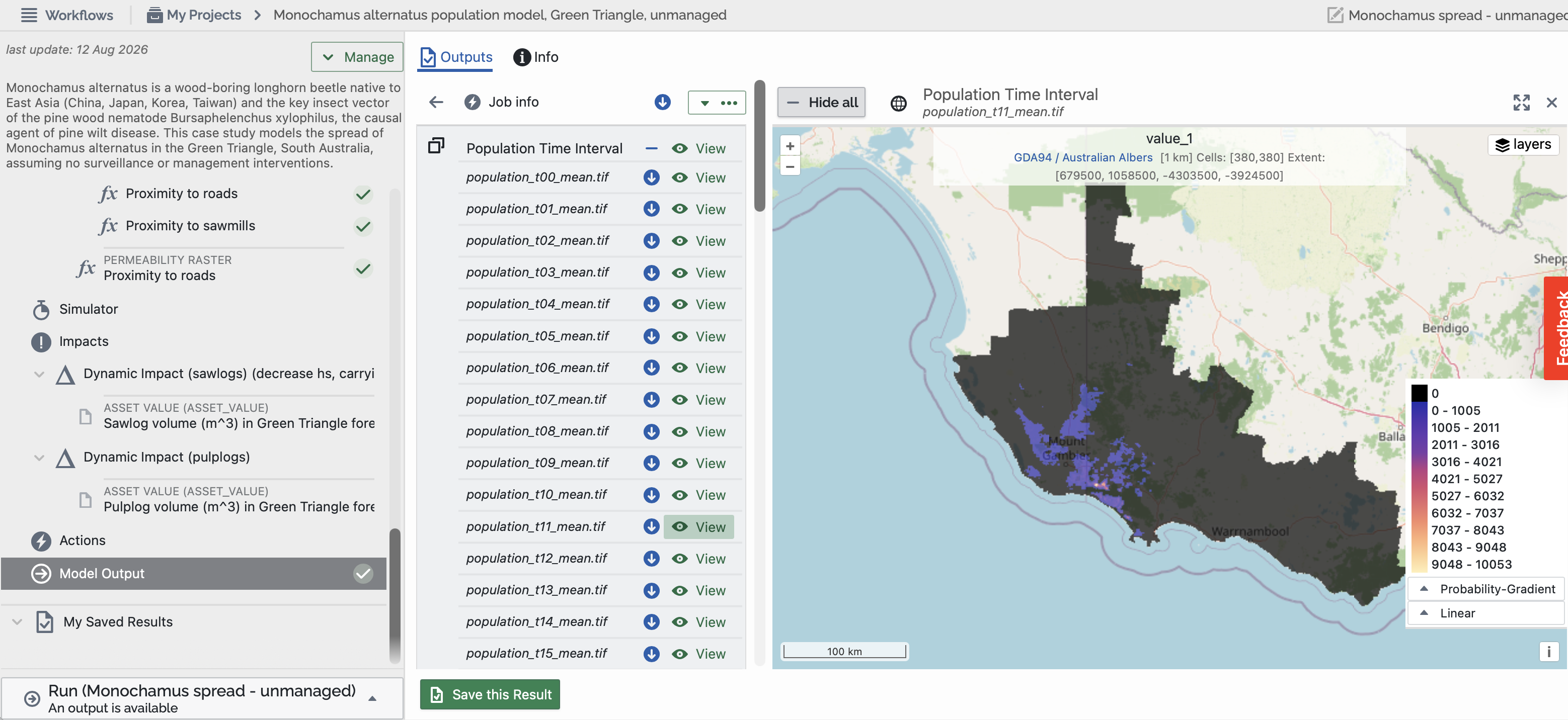
This output will now be discoverable in the users “My results” database, which in turn, makes the layer available for use in other workflows.

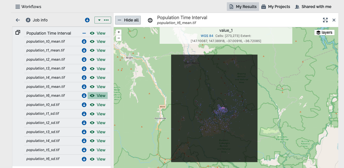
Was this article helpful?
That’s Great!
Thank you for your feedback
Sorry! We couldn't be helpful
Thank you for your feedback
Feedback sent
We appreciate your effort and will try to fix the article