Kernel Estimator

Kernel Estimator is an analytical tool used to quantify how the risk of disease transmission declines with increasing distance between epidemiological units. It applies maximum likelihood estimation to commonly collected temporal epidemiological data—such as the date of onset of clinical signs in animals on an infected premises—to fit and compare a range of alternative kernel functional forms, identify the best-supported model, and infer the probability of infection as a function of distance from known infected premises.

The risk of infection for a susceptible premises is assumed to depend on the amount of “infection pressure” it receives from all infectious premises and is mapped as an output of the tool.

Because data are often limited early in an outbreak, infection pressure is approximated using only a distance-based kernel. The infection pressure on a susceptible premises [MATHS] at time [MATHS] is:

[MATHS]

In simple terms:

• We sum contributions from all infectious premises [MATHS]
• Each contribution depends on the distance [MATHS]
• Closer infected premises contribute more, based on the kernel [MATHS]

Where:

• [MATHS] : infection pressure on premises [MATHS] at time [MATHS]
• [MATHS] : set of infectious premises at time [MATHS]
• [MATHS] : function describing how transmission risk declines with distance

To improve interpretability, infection pressure is standardised by comparing it to the median across all susceptible premises at time [MATHS]:

[MATHS]

In simple terms:

• The infection pressure at each premises is compared to the “typical” (median) value
• A log base 2 scale is used to make differences easier to interpret.

The result [MATHS] represents relative infection pressure:

• [MATHS] : equal to the median risk
• [MATHS] : higher than typical risk, where for example [MATHS] implies the infectious pressure is double that of the median value across all susceptible premises in the input data.
• [MATHS] : lower than typical risk, where for example [MATHS] implies the infectious pressure is half that of the median value across all susceptible premises in the input data

Where:

• [MATHS] : set of susceptible premises at time [MATHS]

The workflow fits a range of commonly used kernel functions to the observed data and estimates their parameters, allowing identification of the function that best represents the underlying transmission process. The term ‘best represents’ refers to the kernel functions achieving the lowest Akaike Information Criterion (AIC) value, a measure of model support that balances goodness-of-fit with model complexity. Currently, the kernel estimator compares the fit of seven commonly used kernels:

• Fat-tailed kernel [MATHS]: A flexible fat-tailed kernel where transmission declines with distance but retains a relatively high probability of long-distance spread.
  Useful when rare long-distance dispersal events are important
• Power law (Type 1) [MATHS]: A simple heavy-tailed kernel with no explicit distance scaling parameter.
  Suitable as a minimal power-law model when scale is implicit in the data
• Power law (Type 2) [MATHS]: A scaled power-law kernel that separates distance scaling and decay rate.
  Commonly used when you want both scale and tail behaviour explicitly parameterised 
• Cauchy [MATHS]: A classic fat-tailed kernel with a strong central peak and substantial long-distance spread.
  A fat-tailed kernel used in epidemiological modelling because it is computationally efficient for large scale studies 
• Exponential (Type 1) [MATHS]: A thin-tailed kernel where transmission declines rapidly with distance.
  Appropriate when spread is highly local with minimal long-distance movement
• Exponential (Type 2) [MATHS]: A less common inverse-distance exponential form that can produce very high short-range transmission and a sharp decline.
  Useful in specific formulations where very strong local transmission dominates
• Exponential (Type 3) [MATHS]: A generalised exponential (Weibull-type) kernel.
  Very flexible for capturing a range of decay behaviours

Linkages to other workflows

Outputs of the Kernel Estimator can be used directly as inputs in many other workflows, such as:

• Informing Spread Modelling by:
  1. Identifying which kernel shape if the best to use for the given context
  2. Estimating the likely daily distance decay kernel based on contemporary or historical incursion data
     Note: Kernels from the Kernel Estimator represent daily transmission risk, and cannot be directly rescaled to longer time steps. To use them at a coarser scale (e.g. monthly), simulate daily transmission over the required period, track the final displacement, and use this to estimate a new kernel for use in spread modelling.
• Informing Surveillance Design by identifying properties of higher relative risk of infection, and thus, where to prioritise additional surveillance resources

Using Kernel Estimator

Step 1. Add Outbreak Data

Kernel Estimator is a simple workflow that requires a single input from users: an outbreak CSV file that contains the following fields:

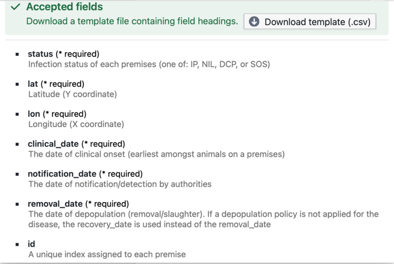
In this CSV, each row should be a separate premises, and all required fields must be specified. Non-infected premises (NIL) are recorded with NA (either the text string “NA”, or an empty string) for all date fields. For infected premises (IP), the date when clinical signs were first observed (clinical_date) is mandatory, with the notification_date added upon official confirmation. Depending on the control policy, such as mandatory depopulation for foot-and-mouth disease (including dangerous contact premises (DCP) or premises on suspicions (SOS)), the culling completion date is recorded in removal_date; otherwise, the date of recovery is entered in recovery_date. The primary objective of this data structure is to estimate the period of infectiousness for each premises (from clinical_date to removal_date or recovery_date), which serves as the basis for estimating the spatial transmission kernel by identifying the duration of infectiousness and the specific premises infected during that period.

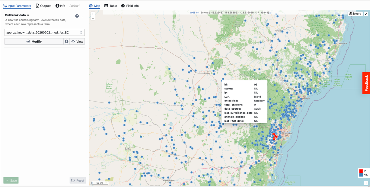
Once the CSV file has been uploaded, point data will be rendered on the map, with the colour scheme identifying infected (IP) vs non-infected (e.g. NIL) premises. Metadata associated with each point can be interrogated by simply zooming in and clicking on the point of interest.

IMPORTANT NOTE:

The reliability of kernel estimation depends heavily on both the number of infected premises (IPs) and the temporal coverage of the data. These models attempt to infer when transmission occurred and over what distance—limited data can lead to highly uncertain results.

While it is technically possible to estimate a kernel with very few IPs or a short time window, such estimates are unlikely to be stable or reliable. In situations where IPs accumulate rapidly over time, reasonable estimates may be achieved with shorter observation periods. However, when detections are sparse or intermittent, longer time series and more observations are required, and even then, results may remain unstable.

As a general guide, users should aim for sufficient sample size and temporal spread before relying on kernel outputs. Based on empirical experience, this often means on the order of ~20 or more IPs across at least a week of observations, although this will vary depending on the outbreak dynamics.

Importantly, users are encouraged to re-estimate kernels regularly as new data become available, and to assess the stability of the estimated parameters over time. Large fluctuations between successive estimates are a strong indication that more data are needed before drawing firm conclusions.

Step 2. Run Model

Users can then run the Kernel Estimator by simply clicking “Run (Kernel Estimator)” in the bottom left-hand corner.

Once completed users will have access to a variety of outputs. 

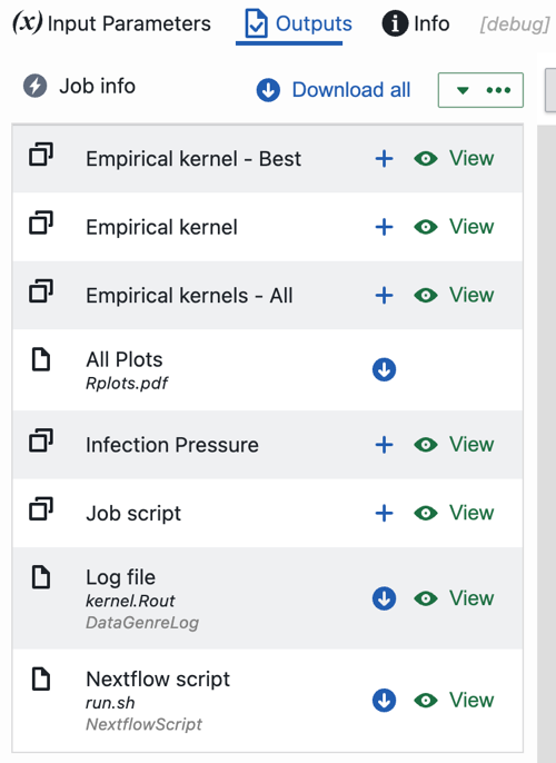
These outputs include:

• Empirical kernel – Best: 
  1. best_kernel.csv: A CSV file of the kernel with the best fit to the data.
  2. best_kernel.png A PNG file showing the fitted kernel.
• Empirical kernel: 
  1. Individual CSV files for all fitted kernels.
• Empirical kernel – All: 
  1. all_kernels.csv: A CSV file containing all kernels.
  2. all_kernels.png: A PNG file showing all estimated kernels.
  3. AIC.csv: A CSV file showing the difference in AIC between each model and the best-fitting model. Also provided is the relative level of support for each model (“weight” column).
• Infection Pressure: 
  1. infection_pressure.csv: A CSV that incorporates all Outbreak data (i.e. input data) columns, but also appends the estimated Relative Infection Pressure and associated Infection Pressure columns derived from the best fitted kernel. Infection pressure is defined as the sum of kernel-derived transmission risks contributed by all active IPs present on the final day of the dataset (excluding previously removed or recovered IPs, DCP, and SOS cases) to each susceptible premises. This value ranges from 0 to [MATHS]. The Relative Infection Pressure refers to the standardised infection pressure, calculated by dividing the infection pressure of each premises by the median infection pressure across all premises, followed by a log transformation. This value ranges from [MATHS] to [MATHS] a value of 0 indicates that the infection pressure for a given premises is equal to the population median.
  2. pointmap.png: A PNG file mapping infection pressure across premises
  3. contourmap.png: A PNG file that plots infection pressure contours.
• Job script: A copy of the R scripts and C++ functions used to build the Kernel Estimator
• Log file: A text file containing processes, messages, and other details associated with model runs
• Nextflow script: A shell script that allows users to rerun models locally via the use of Nextflow and Docker
• Metadata: A .json file containing the metadata required to run the model on Biosecurity Commons
• Input parameters: Input parameters required to run the Job Script

Users may visualise individual kernels by clicking View beside the kernel of interest in the “Empirical kernel” section. An interactive chart will then be shown:

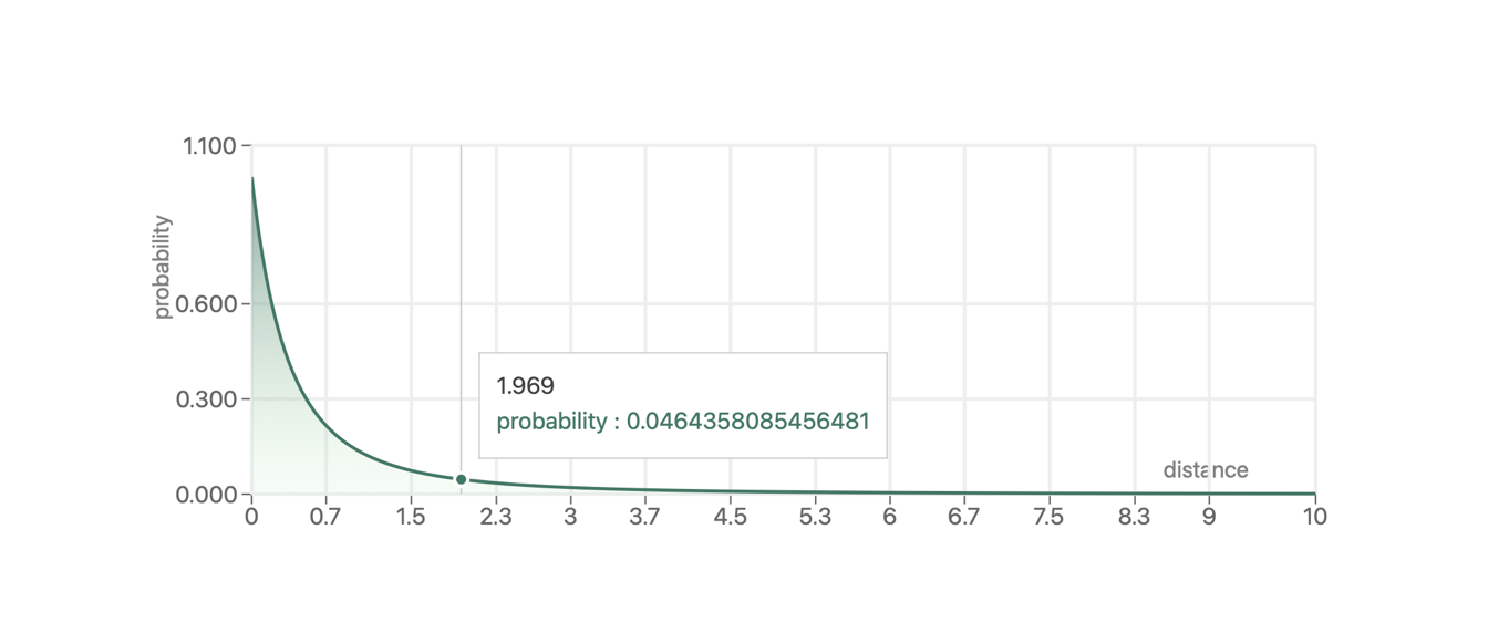
It is important to note that these kernels are best interpreted as daily transmission rates. In addition, some kernel fitting procedures may not converge, and therefore not all kernel outputs are guaranteed to be produced.

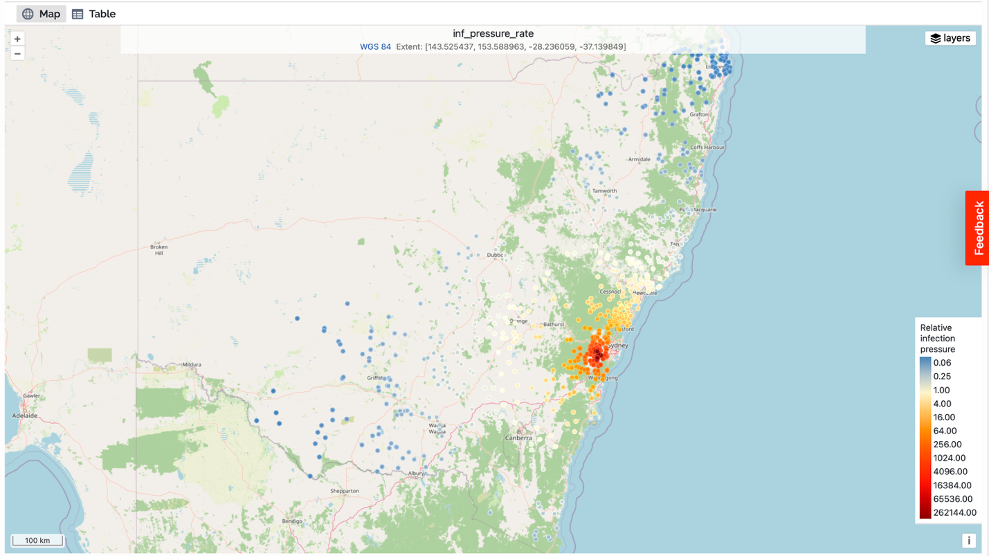
Similarly, users can visualise infection pressure outputs interactively by clicking “View” on infection pressure:

Step 3. Exporting outputs for use in other workflows

Users may wish to export outputs for use in other projects or other workflows.

To do this, view the kernel output, and select “Export to My Results” in the bottom left corner of the interactive map.

This output will now be discoverable in the user’s “My results” database, which in turn makes the layer available for use in other workflows.