Spatial Toolkit

The Spatial Toolkit workflow offers users a range of spatial manipulation tools that can be utilised in a customisable workflow for handling spatial data, including raster and point data. 

This workflow is especially beneficial for preliminary data manipulation before integrating data into other workflows.

For instance, users can create buffers, generate alpha or convex hulls around known points of incursion or infection, transform or normalise rasters, and create new spatial layers by merging multiple rasters or developing distance decay rasters. This workflow enables users to combine multiple toolkit functions, allowing for the creation of a tailored workflow for spatial datasets.

The types of manipulation functions will continue to grow as need arises. 

If there is a manipulation function that you believe will be useful for the broader userbase, please send an email to support@biosecuritycommons.org.au.

Create a Spatial Toolkit project

Step 1. Create a new project

Select the Spatial Toolkit workflow and then select “Create new Project” (see screenshot below).

When creating a new Spatial Toolkit project, users can start an empty project, initially titled “Spatial Toolkit”, which can be renamed appropriately.

The empty project contains the basic structure of the workflow and no preloaded datasets.

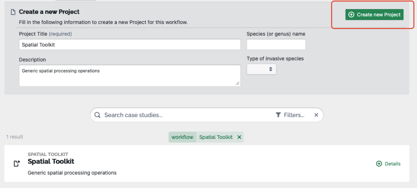
Give your project an appropriate title. You can optionally provide additional descriptive details under the Description, Species name and Species type fields.

Once details have been provided, click the green “Create new Project” button in the bottom right-hand corner to continue.

When you start a Spatial Toolkit workflow you will be presented with the core elements of the on the left side of the screen: “Region” and “Toolkit”. 

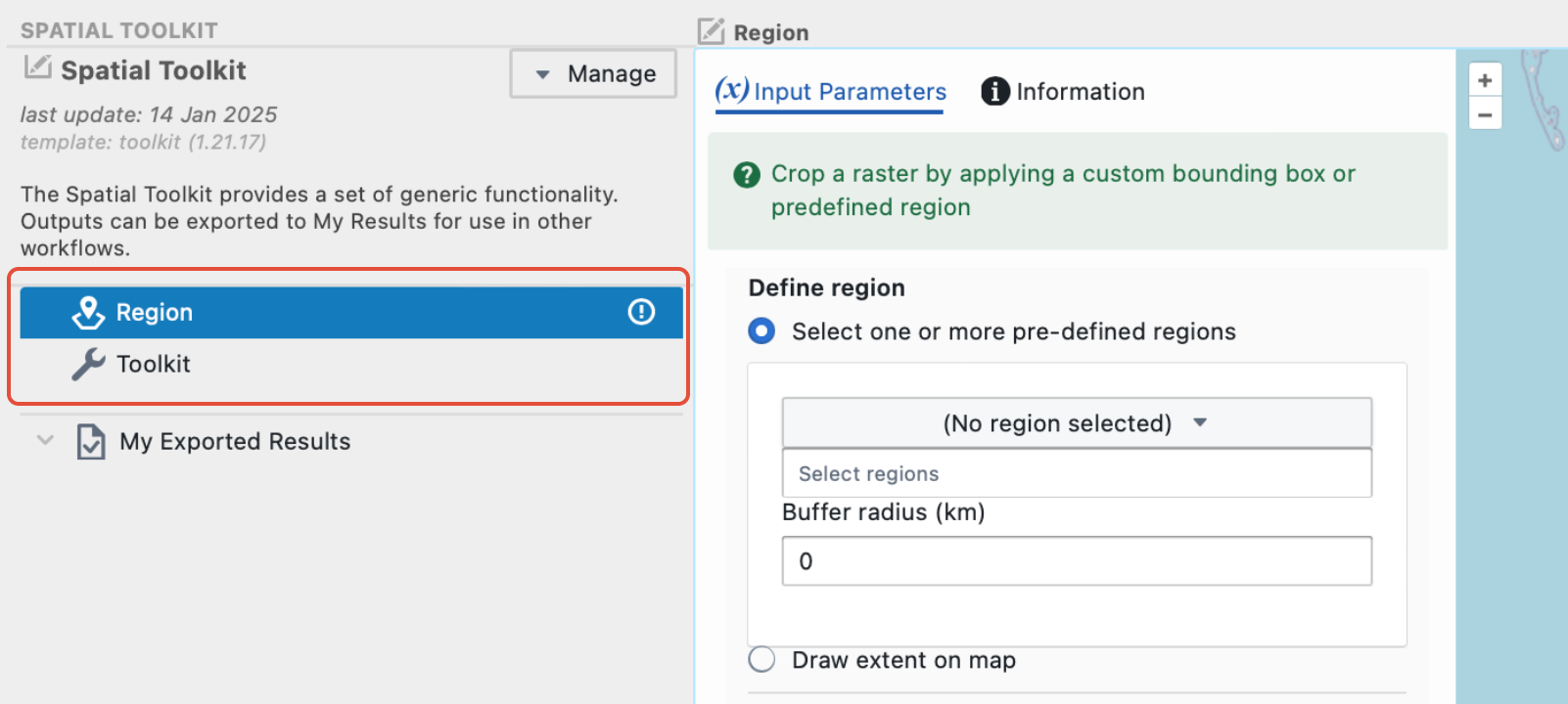
Orange exclamation points indicate steps that require attention and, as you progress through the project, these change to green ticks when complete.

Step 2. Specify your region

Like all other workflows, users can specify the study region using the following approaches:

• Use a template raster
• Use a pre-defined sub-region 
• Manually draw an extent

1. Use a template raster

By default, the Study region will be specified by the “Region Template” - a raster that defines the resolution and extent of the region of interest.

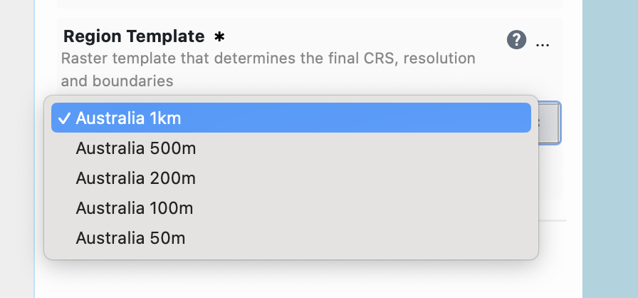
On Biosecurity Commons the default layer is a 1km Australian Albers (equal area) projection layer. Users can select a finer Australian Albers template from the dropdown menu.

Alternatively, if users wish to use a different extent (e.g. different country) or coordinate system, they can replace the default raster by clicking “Add New Input” and select a raster with the desired extent, coordinate system and resolution either from previously uploaded datasets or results, or from existing curated datasets, or else upload a new raster for this purpose using the import/upload option.

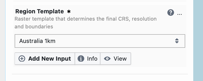
To do this simply select “Add New Input” menu, users have several ways to choose their own study region raster (see screenshot below).

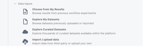
• Choose from My Results: Choose a study region from your results if you have completed previous projects
• Explore My Datasets: To search for datasets you have previously uploaded. This will load a window allowing you to search through datasets you have previously uploaded. Once the relevant dataset is selected, simply click “Select” to the right of the dataset, and then click the green “Add” button in the bottom right of the screen
• Explore Curated Datasets: Search the curated datasets available on Biosecurity Commons. Given the vast number of datasets provided by the platform, we strongly recommend using the filtering functionality to navigate for appropriate datasets. Once the relevant dataset is selected, simply click “Select” to the right of the dataset, and then click the green “Add” button in the bottom right of the screen
• Import/Upload data: Use this option to upload your own study region in GeoTIFF format. Select this option and then select “Upload my own data”. Select your data type and then choose the file you want to upload. Click the green “Next” button and then you will be required to add a title, description, and information regarding the rights associated with the dataset. Finally, click “Finish” and your dataset will be imported. Select the uploaded dataset and then click the green “Add new Input” button

2. Use a pre-defined sub-region

Users may additionally define a study region using one of several pre-defined Australian regions from the drop-down menu. Pre-defined regions include:

• Local Government Areas
• National Resource Management Regions (NRMs)
• Australian state and territories
• IBRA regions
• River regions
• Drainage Divisions (Level 1 or 2)
• Marine Ecoregions of the world
• IMCRA provincial or meso-scale bioregions

For more details about these and other datasets please consult the Atlas of Living Australia. 

Once selected, users can then specify one or more subclasses to define their study region. For example, if a user selected “Australian States and Territories” and they wished to constrain their study region to Queensland, they can simply select it from the dropdown menu.

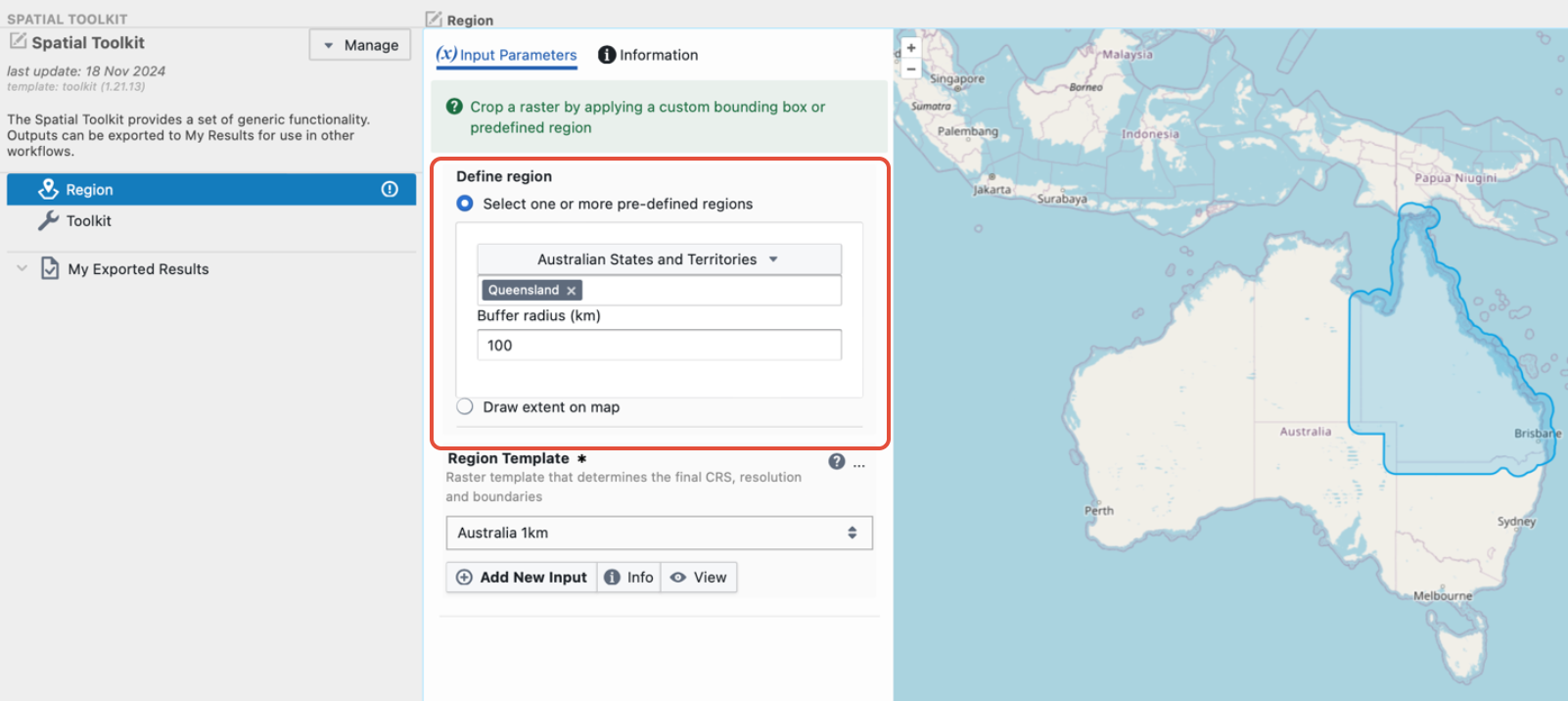
Users can also add a buffer (units in km) to their pre-defined regions. Adding a buffer can sometimes be useful to ensure complex boundaries (e.g. coastlines) are appropriately captured within the study region. 

A “Region Template” is still required as this defines the coordinate system and resolution used to rasterise the chosen study region (see option 1 above for details on how this can be specified).

3. Manually draw an extent

Where a predefined region is not available users can manually draw their extent on the provided map. To do this, select “Draw extent on map”. Users can then either draw a box around the region of interest or draw their own complex polygon over the region of interest. 

Simply specify the draw mode (“Box” or “Poly”) required, then press “Start Drawing”. Then draw your extent on the map provided. If you wish to undo a drawing, simply press “Clear”.

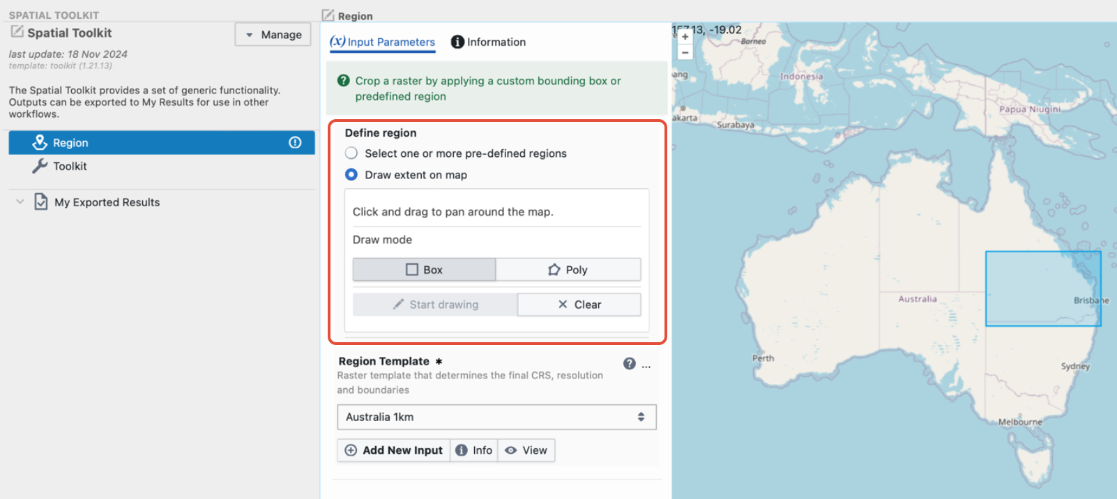
A Region Template is still required as this defines the coordinate system and resolution used to rasterise the chosen study region (see option 1 above for details on how this can be specified).

4. Run the step

When you have made your selections, you will need to save and run this step.

First click on the green “Save” button. 

After the project has saved, the “Run” button on the left-hand side will also turn green. 

Click this button to run the step. 

The output page will be updated as the job progresses from “Created”, “Submitted”, “Started” and “Success”.

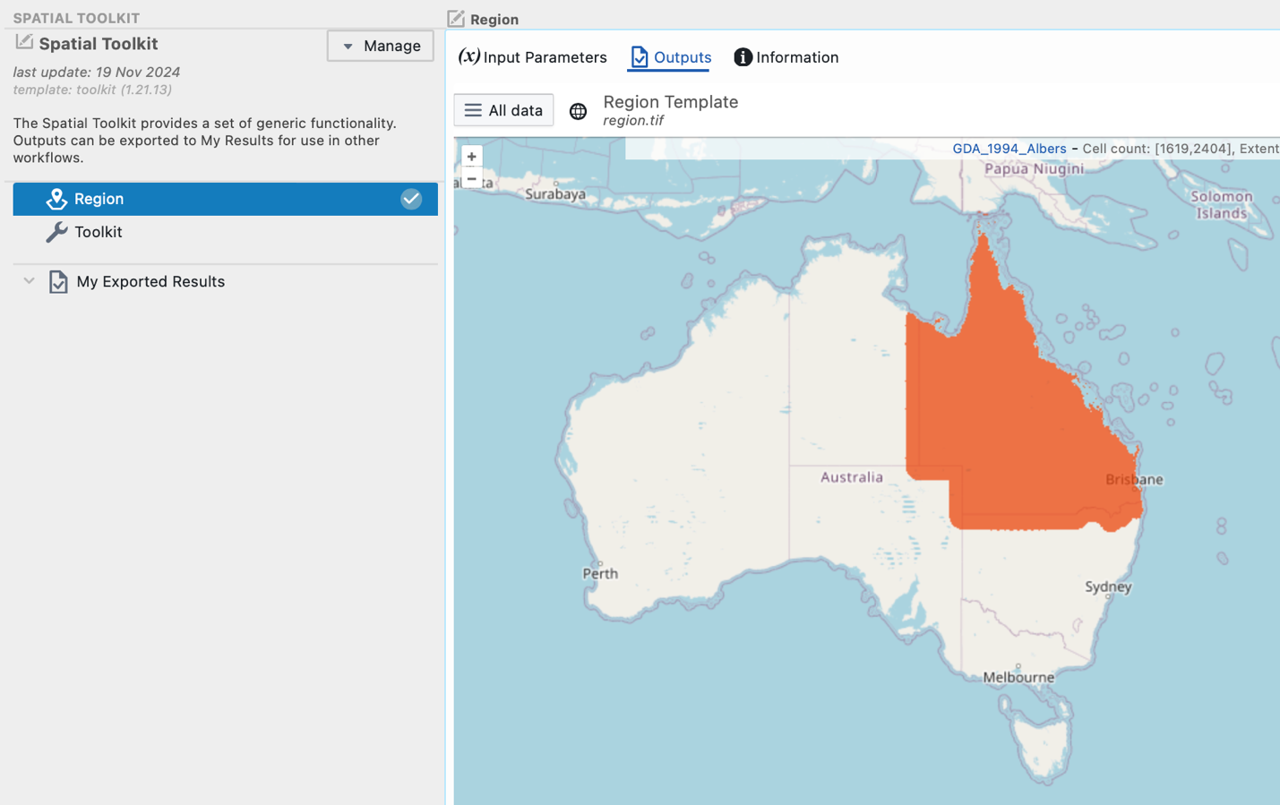
Once it has finished, a green tick will appear next to the Region step in the tree on the left-hand side and your result will look like the example in the screenshot below.

Step 3. Toolkit

The Toolkit branch is where users can select one, or more, GIS manipulation functions.

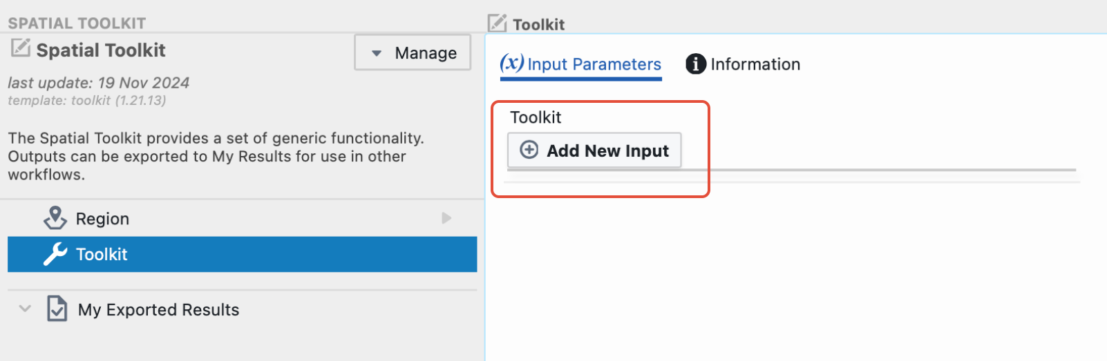
Click on “Add New Input” (screenshot below) and you will be presented with a menu of different options (see second screenshot below).

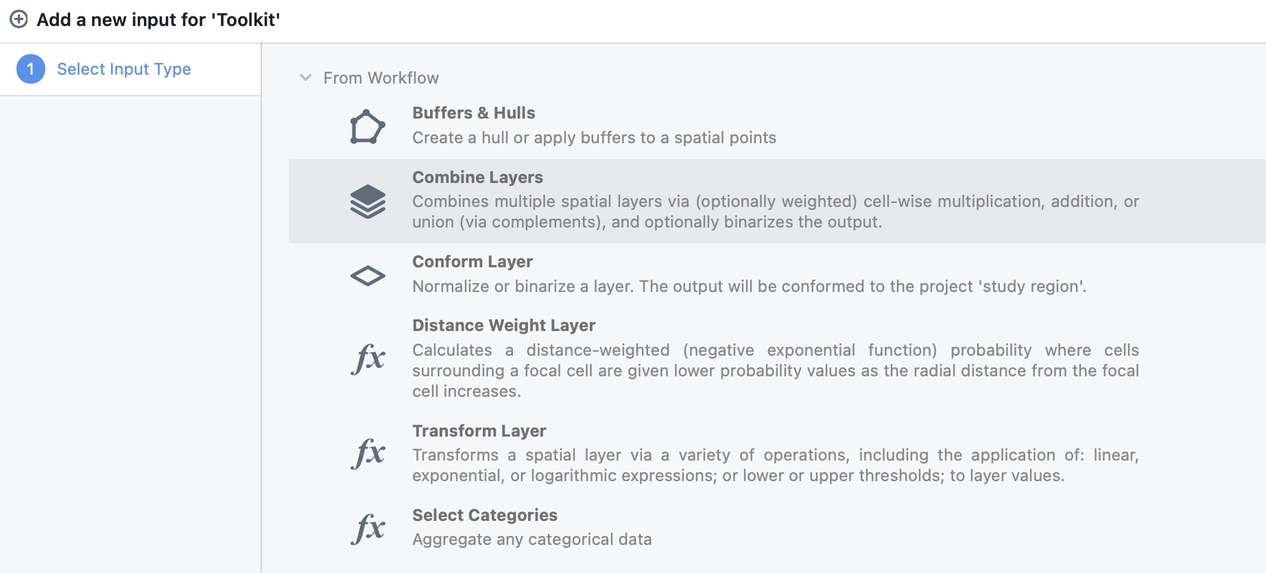
Users can choose from the following options:

• Buffers & Hulls: Useful for adding buffers to spatial data points or constructing alpha or convex hulls around spatial points
• Combine Layers: Useful for combining multiple rasters via (optionally weighted) cell-wise multiplication, addition or union. Also allows output to be binarized if required
• Conform Layer: Useful for binarizing rasters (>0 = 1, <=0 = 0) or normalising a raster based on minimum and maximum values
• Distance Weight Layer: Useful for constructing a distance decay weight raster as a function of spatial point data or pre-calculated distance rasters
• Transform Layer: Useful for conducting linear, exponential, logarithmic transformations or thresholding raster objects
• Select Categories: Useful for selecting categories in categorical rasters (e.g. landuse type, vegetation type), which then can be aggregated and/or binarized to the spatial resolution specified in “Region”

When an option is selected it will appear as a new sub-step in the workflow tree on the left-hand side. 

1a. Buffer and Hulls

Click on the “Buffers & Hulls” sub-step in the tree and you will see the options in the screenshot below.

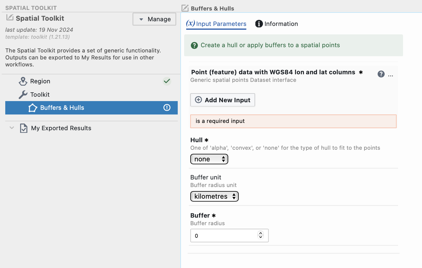
• Point data: A .csv that contains (as a minimum) “lat” and “lon” columns
• Hull: Whether to construct a hull (default = none). Hull options are:
  1. Convex hulls; or
  2. Alpha hulls– if selected, users must also specify an alpha parameter. 
     • alpha parameter controls the level of detail in the shape of the hull, with smaller values creating tighter, more complex shapes around the data points, while larger values produce simpler, more generalized shapes
• Buffer unit: The units used to specify the Buffer parameter. Can be Kilometres or Metres
• Buffer: The numeric radius of the buffer to be applied. Units of buffer radius specified in buffer unit. Default = 0 (i.e. no buffer)

1b. Combine Layers

Click on the “Combine Layers” sub-step in the tree and you will see the options in the screenshot below.

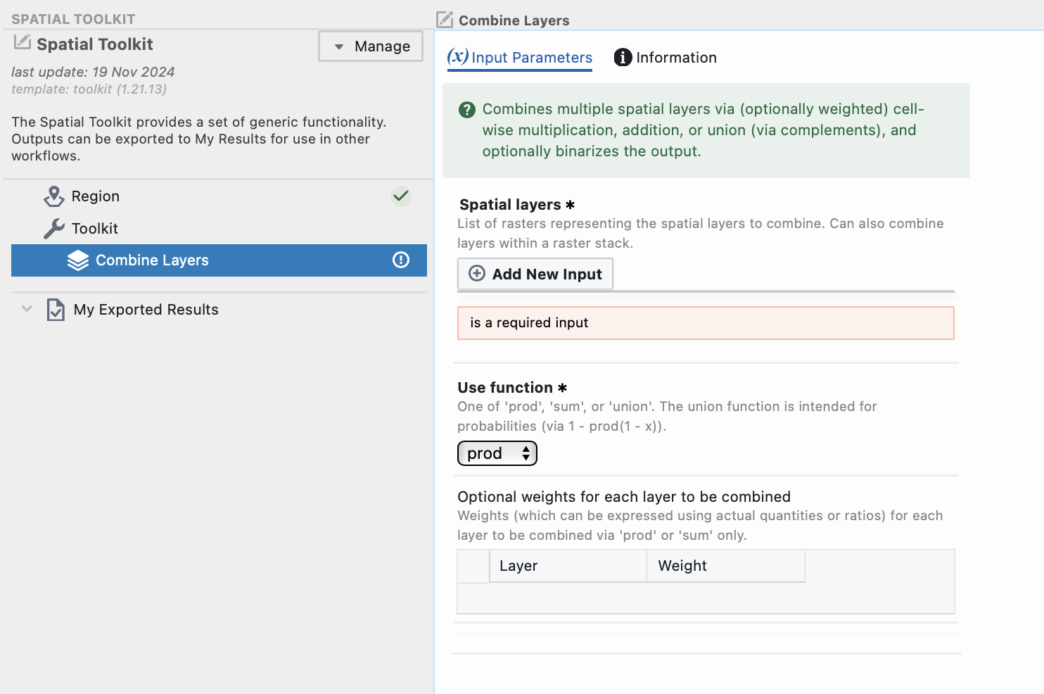
• Spatial layers: Multiple raster objects to be combined. Layers are added one at a time using the “Add New Input” button
• Use function: How should rasters be combined? Options include:
  1. Prod: cell-wise multiplication across rasters
  2. Sum: cell-wise summation across rasters
  3. Union: cell-wise probabilistic union using (1 – prod(1-x)). Useful for combining probability rasters
• Weights (optional): Optional weights that can be applied to each layer. Only applicable to sum and prod combine functions

1c. Conform Layer

Click on the “Conform Layer” sub-step in the tree and you will see the options in the screenshot below.

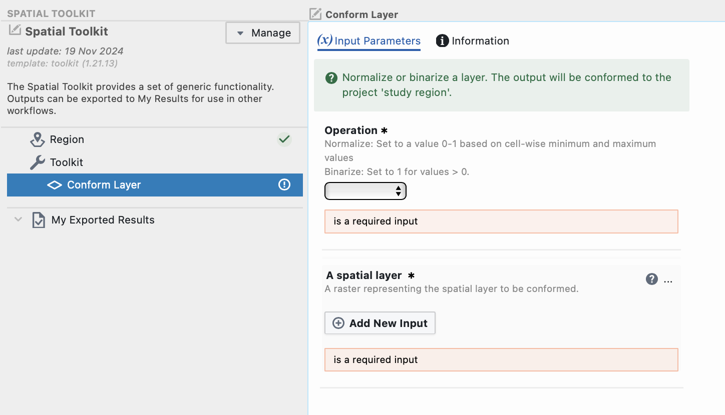
• Operation:Select what conforming operation to perform. Options include:
  1. Normalize: converting raster cell values to between 0-1 by undertaking a normalisation using cell-wise minimum and maximum values
  2. Binarize: Create a binary (0,1) raster where all cell values > 0 are converted to 1 and all values <=0 are converted to 0
• A spatial layer: The raster object to conform

1d. Distance Weight Layer

Click on the “Distance Weight Layer” sub-step in the tree and you will see the options in the screenshot below.

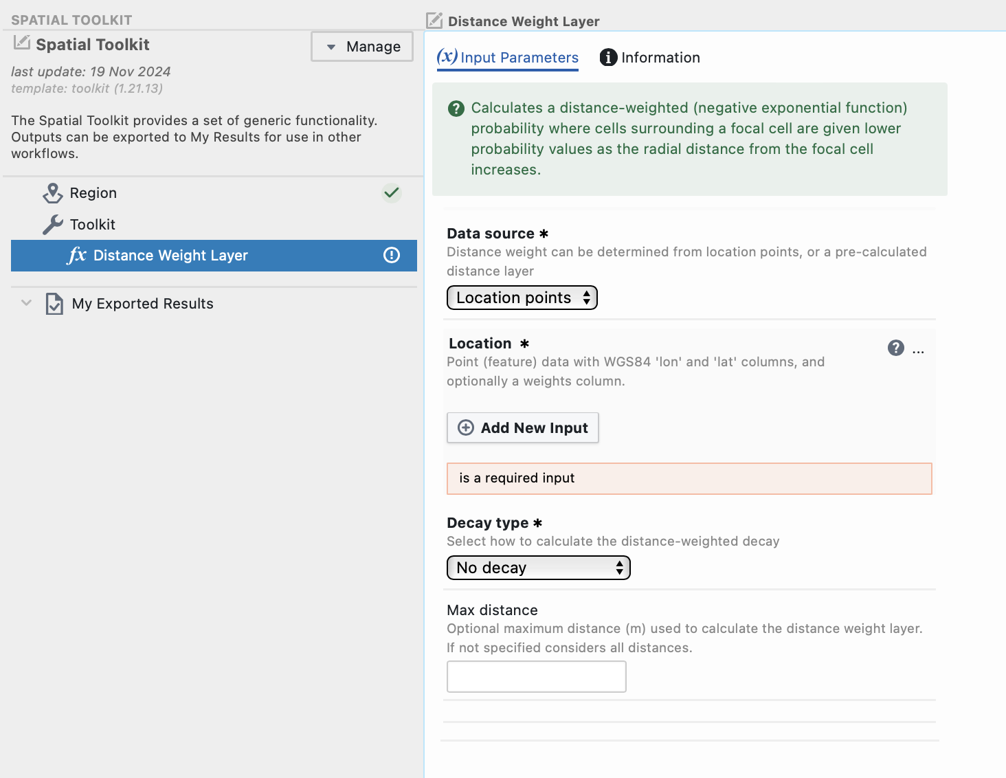
• Data source:
  1. Location points:Specify the locations in which to calculate distance and apply weights. If selected, “Location” must be provided
     • Location: A .csv that contains (as a minimum) “lat” and “lon” columns. But also allowing other optional columns such as “name” and “weight”
  2. Distance layer: Supply a pre-calculated raster of distance from relevant locations. If selected, “Distance raster layer” and “Unit for distances” must be specified
     • Distance raster layer: A raster of pre-calculated distances
     • Unit for distances: Specify the unit scale to use. Options include kilometres or metres 
• Decay type: Two options are available for specifying a negative exponential distance decay:
  1. Half decay: Numeric value. Specify the distance in which half the risk is dispersed. For example, a half-decay value of 20,000m means that 50% of the risk is dispersed within 20,000m (200km) of the locations. If location points are specified, distance units must be in metres. If “Distance” layer is specified, units must be the same as specified in “Unit for distances”
  2. Beta: Numeric value. Specify the beta parameter for the negative exponential function: exp(distance*beta), which transforms cell-to-nearest-point or pre-calculated distances (m) to distance-weighted cell values. Here, beta=log(p)/d (e.g. to have 50% of the likelihood distributed within 20,000m use: log(0.5)/20000 = -0.0034657)
• Max distance (optional): Specify a maximum distance (in m) in which distance decay weights are applied. Default = decay function is applied to all distances available in study region
• Weights (optional): Numeric vector of weights for each point (feature), or character name of column or attribute in “location”, that contains weight values for each point, such that the distance-weighted cell values will be additionally proportionally weighted

1e. Transform Layer

Click on the “Transform Layer” sub-step in the tree and you will see the options in the screenshot below.

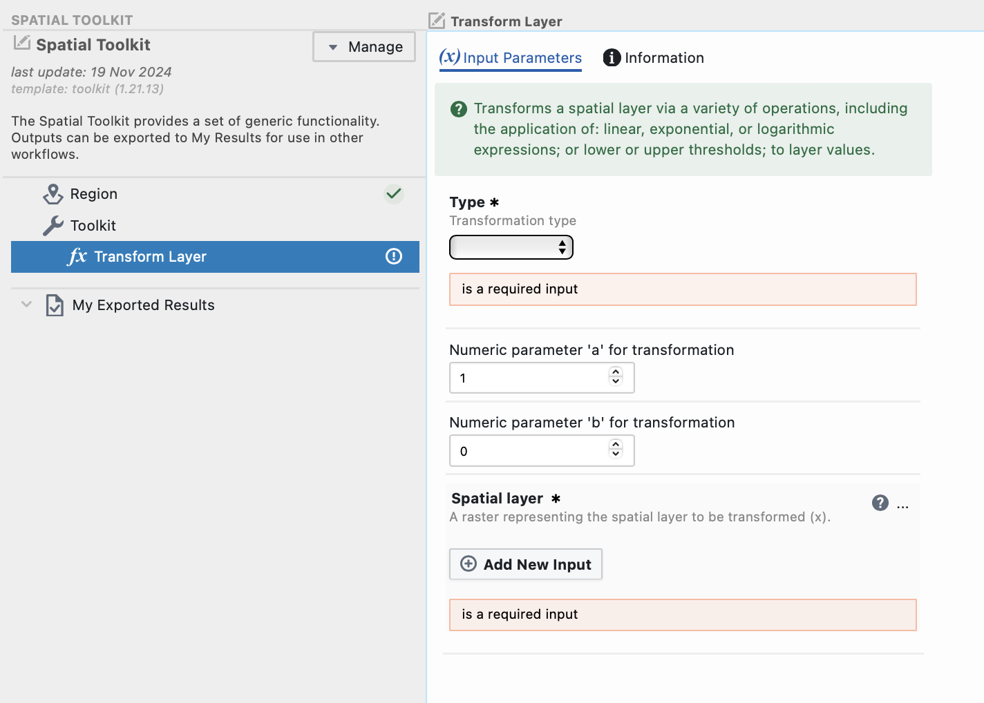
• Type: Generic transform functions. Options include:
  1. Linear: Apply cell-wise linear transformation (a*x + b) to a raster values by specifying parameters “a” and “b”
  2. Exponential: Apply cell-wise exponential transformation (a^x*x^b) to raster values by specifying parameters “a” and “b”
  3. Logarithmic: Apply cell-wise logarithmic transformation, log(x, base = b), by specifying parameter “b”. Default of NULL = natural logarithm (i.e. log(x, base = 2.718)
  4. Lower: Assign all values below a threshold to a value (i.e., x[x < a] = b) by specifying the threshold (“a”) and the replacement value (“b”)
  5. Upper: Assign all values above a threshold to a value (i.e., x[x > a] = b) by specifying the threshold (“a”) and the replacement value (“b”)
• Spatial layer: The raster object to transform

1f. Select Categories

Click on the “Select Categories” sub-step in the tree and you will see the options in the screenshot below.

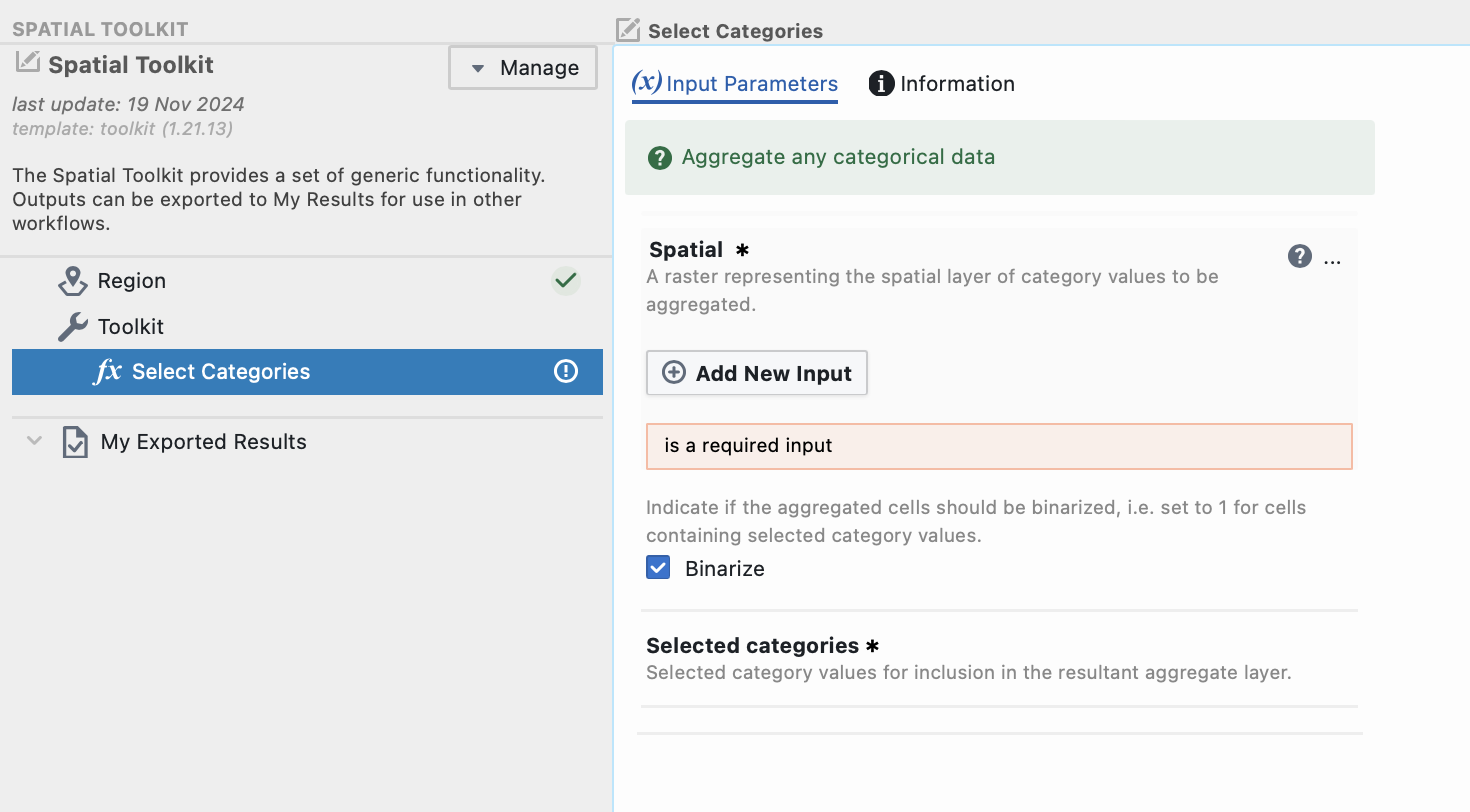
• Spatial: A categorical raster
• Selected categories: Assuming a categorical raster has been uploaded to Spatial, a table of categories will be populated and allow users to select categories (via ticking check boxes) they wish to include and/or aggregate to the spatial resolution and extent of specified in “Region”.
  
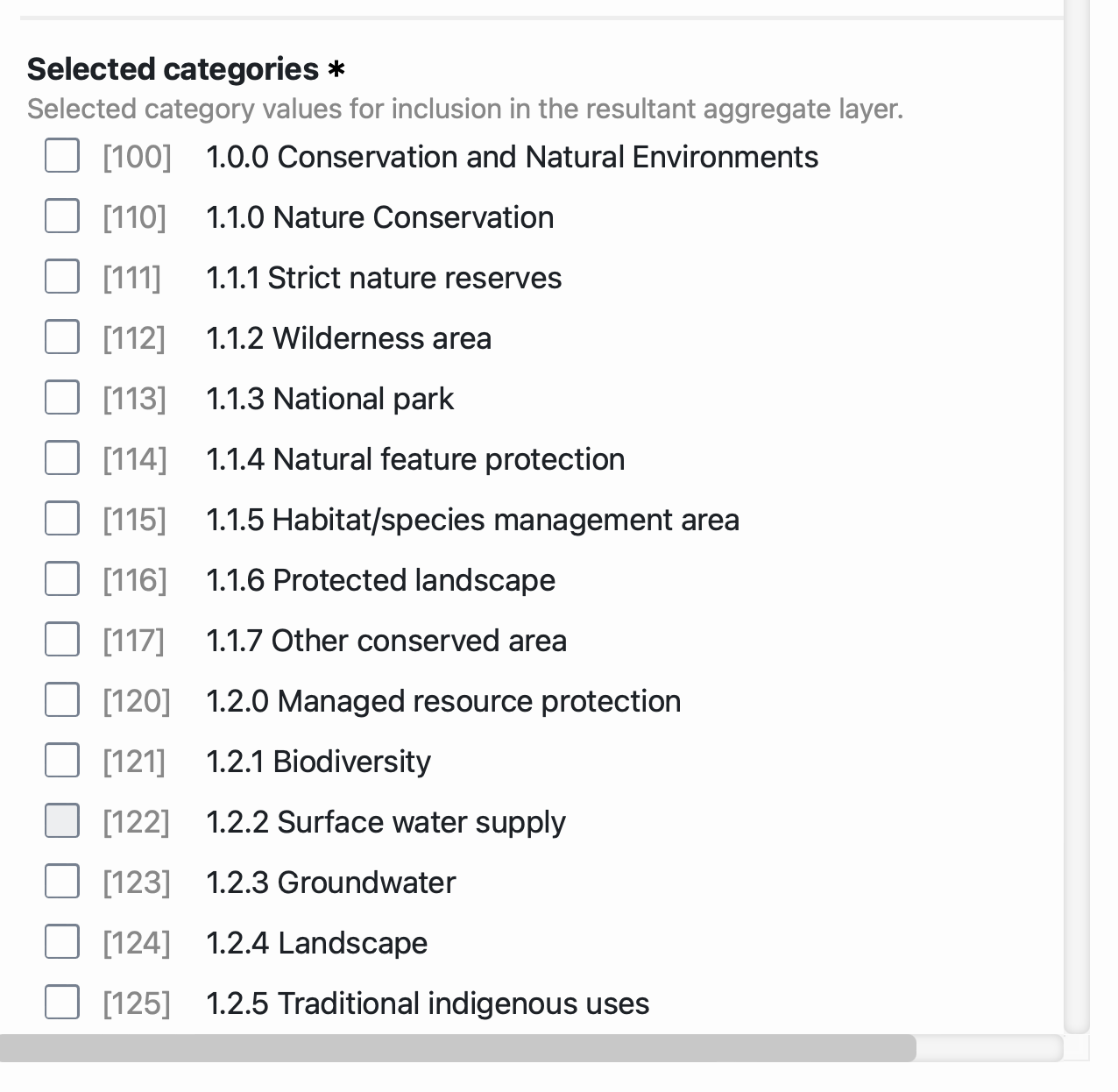
• Binarize: Indicate if cells being aggregated should be binarized (i.e. any sub-cell containing a selected category will result in the aggregated cell being defined as 1 and otherwise zero). Default = TRUE/Checked. If FALSE/unchecked, the proportion of the cell containing suitable categories will be returned. This only applies if the specified region contains a coarser resolution than the categorical raster

2. Run the step

When you have selected the required toolbox function and specified all required parameters, you will need to save and run this step.

First click on the green “Save” button. 

After the project has saved, the “Run” button on the left-hand side will also turn green.

Click this button to run the step.

The output page will be updated as the job progresses from “Created”, “Submitted”, “Started” and “Success”.

Once it has finished, a green tick will appear next to the Toolkit step in the tree on the left-hand side.

3. Create custom workflows by nesting toolbox functionality

The Spatial Toolkit workflow enables users to create custom workflows by combining multiple toolbox functions, which is especially helpful when several operations are needed to produce a specific spatial layer.

For instance, if you want to normalize a raster but first need to apply a threshold, you can easily nest toolbox functions. Start by adding a “Conform Layer” toolbox function to set up the normalization of the raster. Instead of selecting an existing raster as “A Spatial Layer,” choose “Add a Toolbox Function” and select “Transform Layer.” This allows you to define a lower threshold and upload an existing raster object for thresholding.

Next, run the “Transform Layer” function to apply the threshold to the raster. After that, run the “Conform Layer” function to normalize the output from the “Transform Layer”. This way, you effectively chain the operations to achieve your desired result.

Step 4. Exporting outputs for use in other workflows 

Users may wish to export outputs for use in other projects or other workflows. 

To do this, view the output of interest, and select “Export to My Results” in the bottom left corner of the interactive map. 

This output will now be discoverable in the user’s “My results” database, which in turn makes the layer available for use in other workflows.