- Overview
- Scope of the workflow
- Measuring control success
- Selecting a Method
- Specify your management type
- Representing the Control Environment
- Occurrence Probability (or Relative Weight)
- Control Parameters
- Control Allocation
- Optimisation Objectives
- Operational Constraints and Costs
- Common Mistakes & Best Practice
- Want to use our R package?
- References
This article is focused on providing a more in-depth understanding of the Resource Allocation workflow. If you are interested in a step-by-step guide on how to use the Biosecurity Commons interface for Resource Allocation please see our Resource Allocation Quick Start Guide.
Overview
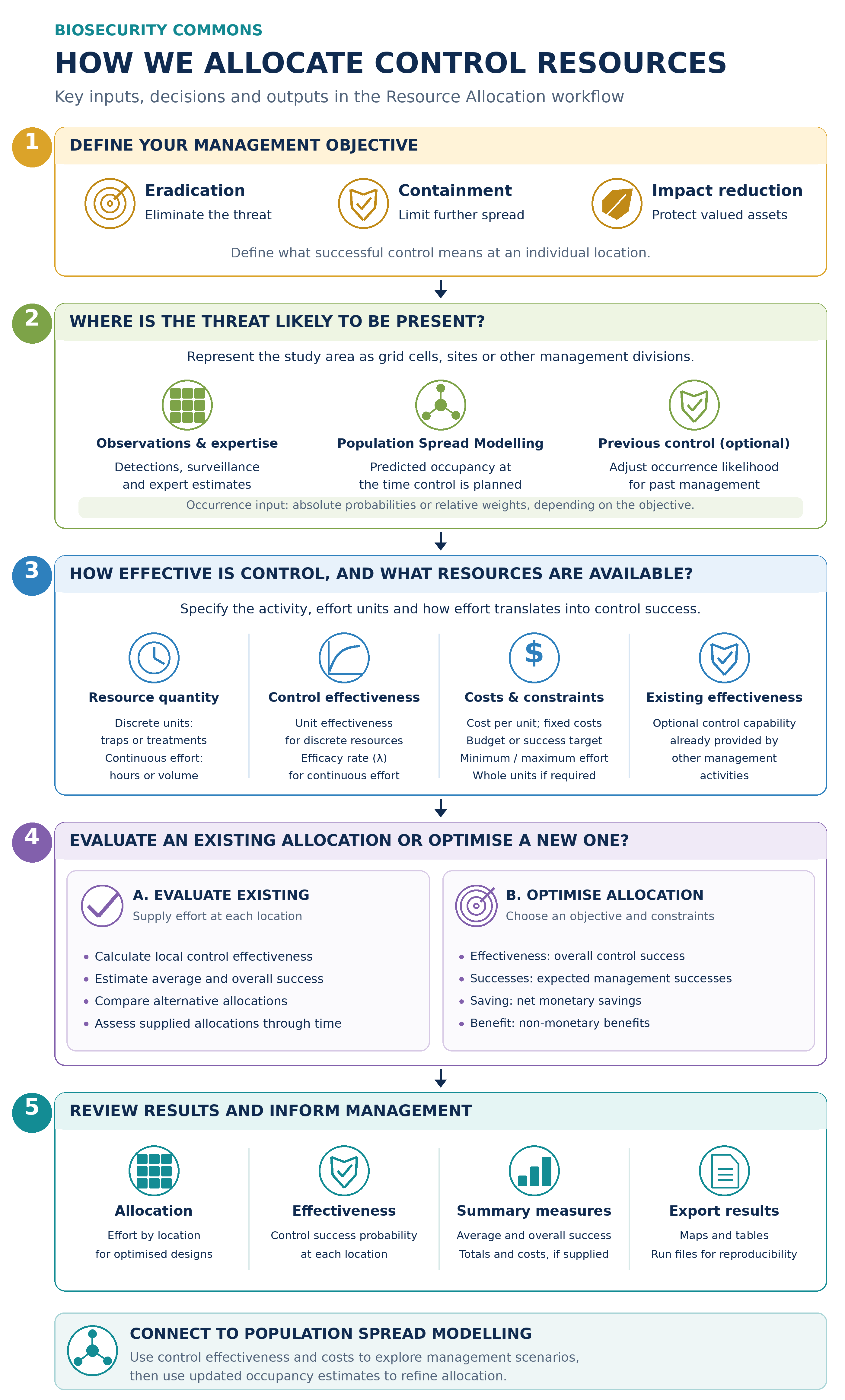
Following a biosecurity outbreak, control activities may aim to eradicate the pest or pathogen, contain its spread, or reduce its impacts on industries, communities and environments. However, funding, personnel and equipment are limited. Decisions about where to intervene and how much control effort to allocate therefore need to maximise progress towards the management objective within the resources available.
The optimal allocation depends on the known or estimated distribution of the threat, the effectiveness and cost of control, and the benefits of successful intervention. An allocation designed to maximise the probability of eradication may differ from one designed to protect high-value assets. Areas with the greatest pest abundance or potential impact will not necessarily offer the greatest benefit from additional control effort.
Biosecurity Commons’ Resource Allocation workflow supports these decisions by relating allocated effort to control effectiveness — the probability of successfully managing the threat at a location, assuming it is present. It combines these estimates with location-specific occurrence likelihoods, costs and benefits to provide two complementary capabilities:
- Evaluate existing control allocations by calculating the probability of successful control at each location, together with average and overall success probabilities across the study region. This allows practitioners to assess current allocations and compare alternative distributions of effort.
- Optimise control resource allocation by identifying where and how much effort should be deployed to best achieve a specified management objective.
Depending on the decision context, optimisation can:
- maximise the overall probability of control success across all occupied locations;
- maximise the expected number of locations where control succeeds;
- maximise net monetary savings, based on the monetary value of successful control minus control allocation costs; or
- maximise a user-defined non-monetary benefit, such as protecting biodiversity or other high-value assets.
Optimisation can be constrained by the available budget, required average or overall probabilities of success, and minimum or maximum allocations at individual locations. The workflow also accounts for costs per unit of effort and fixed deployment costs, such as travel or site establishment. Existing control effectiveness and information about previous control can inform the allocation of additional resources.
The optimisation uses generalised Lagrange-based approaches described by Hauser & McCarthy (2009), McCarthy et al. (2010), Giljohann et al. (2011) and Moore et al. (2016), together with relationships describing how control effectiveness increases with effort.
Scope of the workflow
The Resource Allocation workflow determines how control effort should be distributed across locations to achieve a specified objective. Users define the control activity and provide estimates of its effectiveness, costs and benefits. The workflow allocates effort for that activity; it does not automatically select between alternative control methods or simulate how treatment changes population growth and spread.
Clearly defining successful control is therefore essential. If the objective is eradication, effectiveness estimates must describe the probability of completely eliminating the threat from a location, rather than simply reducing its abundance. For other objectives, the definition of success and the benefits assigned to it should reflect the intended management outcome.
Potential spread and damage can inform the benefits assigned to successful control, but these consequences must be estimated outside the allocation calculation. Results should therefore be interpreted in light of the supplied inputs and assumptions.
How does Resource Allocation differ from Surveillance Design?
Resource Allocation shares many of the optimisation approaches and inputs used in the Surveillance Design workflow. Both account for occurrence likelihood, effort-dependent effectiveness, costs and operational constraints.
The key difference is the outcome being optimised: Surveillance Design focuses on detecting the threat, whereas; Resource Allocation focuses on successfully managing it. This distinction concerns the purpose of the activity rather than its timing, because surveillance and control may both be required during an outbreak response.
For surveillance, detecting the threat at any one location is sufficient to achieve a system-wide detection. By contrast, for control, system-wide success requires successful management at every occupied location. Consequently, an allocation designed to maximise detection probability may differ substantially from one designed to maximise control success across an outbreak.
Control success probabilities also serve a different purpose from surveillance sensitivity. They describe expected management outcomes; they do not directly quantify confidence in pest absence following zero detections.
Measuring control success
The workflow calculates the probability of successful control at each location and summarises performance across the study region using two measures:
- Average probability of control success: the average of the location-specific success probabilities, weighted by the likelihood that the threat occurs at each location.
- Overall probability of control success: the probability of successful control at every occupied location, conditional on the threat being present somewhere in the region and under the model’s assumptions.
A high probability of success at individual locations does not necessarily imply a high probability of controlling the entire outbreak. For example, if the threat occurs at ten locations and control has a 90% probability of success at each, the average probability is 90%. Assuming independent outcomes, however, the probability of success at all ten locations is only about 35% (0.9¹⁰).
The appropriate measure depends on the management objective. The average describes performance across locations, while the overall probability is relevant when success requires controlling every occupied location, as in eradication.
Relative occurrence likelihoods can be used to calculate the weighted average and optimise expected management successes or non-monetary benefits. Actual occurrence probabilities are required for monetary savings optimisation and for calculating or optimising the overall probability of control success.
Selecting a Method
Biosecurity Commons currently provides one resource allocation method: Control Design. This method helps users evaluate existing control allocations or optimise how control resources are distributed across spatial locations or other management divisions, such as species or invasion pathways.
For optimisation, Control Design uses Lagrange-based methods to identify allocations that maximise management success, net monetary savings or non-monetary benefits, subject to specified operational constraints. For existing allocations, it calculates the probability of control success at each location or division and summarises effectiveness across the study region.
Control effort can be represented as either continuous quantities, such as control hours or treatment volume, or discrete units, such as traps or treatments. Users specify how the amount of effort allocated translates into the probability of successful control.
Future updates are intended to introduce additional optimisation methods, including portfolio analysis (Kompas et al 2019), to help allocate resources across multiple threats or activities spanning pre-border, border and post-border biosecurity.
Specify your management type
The first step in developing a resource allocation model is to define what resources will be allocated and how they will be measured. Biosecurity Commons asks users to specify the resource type (e.g. survey, trap, treatment, removal, mixed resource or other) and the resource quantity unit (e.g. hours, traps, treatments, removals or units).
These inputs describe the allocation and do not directly affect the model calculations. They help clarify the management activity being planned and inform the subsequent choice between continuous effort, such as control hours or treatment volume, and discrete resources, such as a count of traps or treatments.
Representing the Control Environment
Biosecurity Commons allows control resources to be allocated across raster grids, spatial locations, or non-spatial management divisions. The appropriate representation depends on whether control is planned across a continuous landscape, a set of individual sites, or other management units.
Raster grids
Raster grids are used when control resources are allocated across a continuous landscape. The study region is divided into regularly sized cells, with the workflow determining how much effort to allocate to each cell. This approach is well suited to landscape-scale control where occurrence likelihood, control effectiveness, costs or benefits vary across space.
For example, predicted occupancy from a population spread model can help identify where control may be required following an outbreak. Raster-based designs produce maps showing the allocation of control effort and the corresponding probability of control success.
Conforming layers to the region raster
When using a raster to define the study region, users can incorporate additional raster layers representing occurrence likelihood, control effectiveness or other inputs. These layers may differ in their coverage or treatment of undefined (NA) cells.
Biosecurity Commons provides two options for filling undefined cells within the defined study region:
- Zero undefined values (default): Sets undefined cells to zero wherever the region raster has a defined value.
- Nearest defined values: Fills undefined cells with the mean value of the nearest cell or cells containing defined values. This can help address small mismatches in borders or coastlines between layers.
The appropriate option depends on what missing values represent. Setting an undefined occurrence value to zero treats the threat as absent from that cell; it does not represent uncertainty about its presence. Similarly, filling gaps from nearby cells assumes those neighbouring values are representative.
Spatial locations
Spatial locations are used when control resources are allocated among sites defined by geographic coordinates, such as farms, orchards, infested properties or treatment sites. The workflow determines how much effort to allocate to each site using its occurrence likelihood, control effectiveness and other relevant inputs.
Other (aspatial) divisions
Control resources can also be allocated across management divisions without geographic coordinates, such as species, invasion pathways or other user-defined categories.
Each division must have an appropriate occurrence likelihood and a defined relationship between allocated effort and management success. Costs, benefits and resource units must also be comparable across divisions so that the resulting allocation has a consistent interpretation.
Occurrence Probability (or Relative Weight)
The Occurrence Probability (or Relative Weight) input represents the likelihood that the target threat occurs within each raster cell, spatial location or aspatial division. The Resource Allocation workflow combines these values with control effectiveness, costs and benefits to determine where intervention is expected to contribute most to the management objective.
For post-outbreak control, this input should generally describe occupancy at the time control is planned. It should account for available evidence about the outbreak’s distribution, including confirmed detections, possible spread and any subsequent control. Depending on the optimisation objective, values can be supplied as absolute occurrence probabilities or relative occurrence weights.
Known infestations and uncertain occurrence
Where the threat is confirmed to remain present, an occurrence probability of 1 can represent known occupancy. Elsewhere, probabilities may be estimated from delimiting surveillance, predictive models or expert elicitation. A location without a detection should not automatically receive a probability of zero, because the threat may be present but undetected.
If occurrence is known at every candidate location, differences in control allocation are driven by control effectiveness, costs, benefits and operational constraints rather than differences in occurrence likelihood.
Using Population Spread Modelling outputs
The Population Spread Modelling workflow can inform occurrence likelihood by predicting where the threat may have spread following introduction. Occupancy estimates for a relevant time step can be used to support the allocation of eradication, containment or suppression effort.
The selected time step should correspond to the period when control is intended to occur. Predicted abundance is not itself an occurrence probability and should not be treated as one without an appropriate conversion. Likewise, using abundance as a relative occurrence weight requires justification: locations with more individuals are not necessarily proportionally more likely to be occupied.
This provides a link between Population Spread Modelling and Resource Allocation. In the other direction, control effectiveness outputs from Resource Allocation can inform management scenarios in Population Spread Modelling.
Using Risk Mapping and other evidence
The Risk Mapping workflow provides information about establishment likelihood based on arrival, abiotic suitability and biotic suitability. These outputs may inform control planning where they are relevant to the management context (e.g. reducing the likelihood of arrival establishment).
However, initial establishment likelihood is different from current occupancy following an outbreak. For post-outbreak control, risk maps should be interpreted alongside evidence about detections, spread and previous management. Habitat suitability alone does not establish that the threat is present.
Occurrence estimates can also draw on field observations, surveillance records, historical detections and structured expert elicitation. Where previous control has already been incorporated into those estimates, it should not be applied again through the workflow’s optional previous-control inputs.
Absolute probabilities versus relative weights
An absolute probability estimates the chance that the threat occurs within a particular cell, location or division. For example, values of 0.20 and 0.80 represent estimated occurrence probabilities of 20% and 80%, respectively.
A relative weight describes occurrence likelihood in proportion to other locations without specifying the actual probability of presence. For example, weights of 10 and 5 represent a twofold difference in occurrence likelihood, provided the weights are proportional to occurrence probabilities. Arbitrary suitability scores or rankings do not necessarily support this interpretation.
The choice depends on the optimisation objective:
- Relative weights can be used to optimise expected management successes or non-monetary benefits, and to calculate the occurrence-weighted average probability of control success. Both the relative magnitudes of the weights and the other model inputs influence the allocation; their ranking alone is insufficient. Without absolute occurrence probabilities, results cannot be interpreted as an absolute expected number of successfully controlled occupied locations.
- Absolute probabilities are required to calculate or optimise the overall probability of control successacross all occupied locations, and to optimise net monetary savings. These calculations depend on the actual likelihood that control is needed, rather than its relative distribution alone.
Accounting for past management activity (Optional)
Control undertaken before the planned allocation may reduce the likelihood that the threat remains present. The optional Previous control parameters account for this by adjusting occurrence likelihood before evaluating or optimising the allocation of further control effort.
Users specify:
- Previous control proportion: the proportional reduction in occurrence likelihood attributed to each previous control application, expressed between 0 and 1. For a single round of control, this is broadly equivalent to the effectiveness of previous control effort (or the probability the control was successful).
- Number of repeats: the number of times that previous control was applied. Values can vary among locations. If not specified one application of control is assumed.
The occurrence likelihood after previous control is calculated as:
where
pa = adjusted occurrence likelihood
p0 = occurrence likelihood before previous control
c = proportional reduction in occurrence likelihood per control application
r = number of previous control applications
For example, an initial occurrence probability of 0.8, with two applications each reducing the remaining occurrence likelihood by 50%, becomes:
This adjustment assumes each application produces the same proportional reduction in the remaining occurrence likelihood. It does not explicitly model population recovery or reinvasion between applications. Because the adjustment acts on occurrence likelihood, a percentage reduction in pest abundance should not automatically be interpreted as an equivalent reduction in the probability of presence.
IMPORTANT NOTE:
If the supplied occurrence estimates already account for previous control, leave these parameters unspecified to avoid counting its effects twice. This option is distinct from existing management effectiveness, which represents control capability already in place and combines with the effectiveness of the allocation being assessed.
The Previous control proportion can be specified in two ways:
1. Effectiveness per application: Enter the proportional reduction in occurrence likelihood attributed to one control application, and set Number of repeats to the number of applications that were undertaken. This assumes each application has the same effectiveness.
2. Combined effectiveness across applications: Enter the cumulative proportional reduction in occurrence likelihood attributed to all previous control activities, and set Number of repeats to 1. This avoids applying the combined effect more than once.
For example, two applications that each reduce the remaining occurrence likelihood by 50% can be represented as either 0.5 with two repeats, or 0.75 with one repeat.
Values must be proportions between 0 and 1. An efficacy rate (for continuous control measures) such as λ must first be converted to an effectiveness probability using the amount of effort applied; it should not be entered directly.
Control Parameters
The Parameters section defines how allocated control resources translate into the probability of successful control at a location, assuming the threat is present. Users first select whether the resource quantity is discrete or continuous, then specify the corresponding effectiveness parameter.
The choice depends on how control effort is measured. Discrete resources are counted as individual units, whereas continuous resources are measured as an amount of effort or material.
Discrete resources
Discrete resources are appropriate when control effort consists of countable units, such as traps, treatment applications or removal operations. The allocation represents the number of units deployed at each location.
The required parameter is unit effectiveness: the probability that one unit achieves the defined control outcome at a location, conditional on the threat being present. Biosecurity Commons calculates the combined effectiveness of n units as:
where
u = unit effectiveness, expressed as a probability between 0 and 1
n = number of control units allocated to the location
For example, if each treatment application has a 40% probability of achieving successful control, three independent applications give:
The resulting probability of control success is 78.4%. This formulation assumes that units act independently and have the same effectiveness within a location. Unit effectiveness can differ between locations.
The definition of unit effectiveness must match the management objective. For example, if success means local eradication, it must represent the probability that one control unit eliminates the local population, rather than the probability of removing a single individual.
Continuous resources
Continuous resources are appropriate when control is measured as an amount that can be divided into fractional quantities, such as control hours or treatment volume. The allocation represents how much effort or material is assigned to each location.
The required parameter is efficacy (λ), which determines how rapidly the probability of successful control increases with allocated effort:
where
λ = efficacy rate per unit of control effort
E = amount of control effort allocated to the location
A larger λ means that less effort is required to achieve a given probability of control success. Unlike unit effectiveness, λ is a rate, not a probability, and is not restricted to values between 0 and 1. Its units must match the effort measure: for example, per hour when effort is measured in hours.
For example, with an efficacy rate of 0.2 per hour and five hours of control effort:
The resulting probability of control success is approximately 63.2%.
Specifying control effectiveness
For either resource quantity type, effectiveness can be supplied as a single value across the study region or allowed to vary among locations or divisions, using a raster or CSV input appropriate to the selected environment.
Estimates should match the control method, resource unit, spatial scale, treatment period and definition of success. Both formulations assume diminishing returns: additional effort increases the probability of success, but each additional unit produces a smaller increase.
Control Allocation
The Allocation section determines whether the workflow evaluates an existing distribution of control effort or optimises a new allocation. Biosecurity Commons provides two options: Existing and Optimisation.
Existing control allocation
The Existing option calculates the effectiveness of a control allocation supplied by the user. Users specify the amount of control effort at each location or division, such as treatment hours, traps or treatment applications.
The workflow combines these quantities with the control parameters to calculate:
the probability of control success at each location, conditional on the threat being present;
the average probability of control success, weighted by occurrence likelihood; and
the overall probability of control success across all occupied locations, where absolute occurrence probabilities are supplied.
This option allows users to assess current control programs and compare alternative allocations. No optimisation is performed: the workflow evaluates the supplied allocation.
Allocations for multiple time intervals (as either a raster stack, or CSV) can also be provided, allowing effectiveness to be assessed for a sequence of control activities.
Optimised control allocation
The Optimisation option identifies how control resources should be distributed to best achieve a selected objective, subject to operational constraints.
The objective determines what constitutes the best allocation. Maximising the expected number of successfully controlled locations, for example, may favour a different allocation from maximising the probability of eliminating the threat from every occupied location.
The following table provides a guide to selecting an objective.
| Management priority | Optimisation strategy | Interpretation |
| Achieve successful control across the entire outbreak | Effectiveness | Maximise the probability of success at every occupied location. Appropriate for eradication planning when success means local elimination. |
| Achieve successful control at as many locations as possible | Successes | Maximise the expected number of occupied locations where control succeeds. |
| Balance control expenditure against monetary benefits | Saving | Maximise expected monetary savings after subtracting control allocation costs. |
| Protect environmental, social or other valued assets | Benefit | Maximise the expected non-monetary benefit of successful control. |
Optimisation Objectives
Maximise overall control success — Effectiveness
This objective allocates resources to maximise the probability of successful control at every occupied location, conditional on the threat being present somewhere in the study region.
It is relevant when success requires managing the entire outbreak. For eradication planning, the control parameters must therefore describe the probability of completely eliminating the threat from each location.
Unlike the Successes objective, which rewards each successfully controlled location, this objective considers whether control succeeds across all occupied locations together. Leaving one occupied location uncontrolled prevents overall success.
Absolute occurrence probabilities are required for this optimisation objective.
Maximise expected management successes — Successes
This objective allocates resources to maximise the expected number of occupied locations where control succeeds. It accounts for both the likelihood that the threat occurs at a location and the probability that the allocated effort will successfully control it.
Under a fixed budget, it may favour locations where successful control can be achieved with relatively little effort. It does not require success at every occupied location and does not directly maximise the number of individual organisms removed.
For a fixed set of occurrence inputs, maximising expected successes also maximises the occurrence-weighted average probability of control success.
Absolute probabilities or relative occurrence weights can be used. With relative weights, the allocation reflects relative priorities, but the result cannot be interpreted as an absolute expected count of successfully controlled occupied locations.
Maximise net monetary savings — Saving
This objective balances the expected monetary benefits of successful control against the costs of allocating control resources.
Users provide a saving value for each location, representing the monetary loss or expenditure avoided if control succeeds there. This may include avoided production losses, asset damage or future management costs. Values should use a consistent currency, time horizon and comparison scenario.
The workflow weights these savings by occurrence likelihood and control effectiveness, then subtracts allocation costs. Users should therefore enter the saving associated with successful control before subtracting the costs of the control allocation being optimised.
The resulting allocation considers where additional effort is expected to generate sufficient savings to justify its cost. If None is selected as the constraint, the workflow seeks this balance without a specified budget or success target.
Absolute occurrence probabilities are required for this objective.
Maximise non-monetary benefits — Benefit
This objective allocates resources to maximise a user-defined measure of benefit associated with successful control, such as protecting threatened species, habitat condition or culturally significant assets.
Users provide a benefit value for each location. Values must be comparable across locations, with larger values representing greater benefits from successful control. Where possible, they should reflect the improvement or avoided loss attributable to control, rather than asset value alone.
The workflow combines these values with occurrence likelihood and control effectiveness. Costs can influence how resources are distributed within a budget, but they are not subtracted from non-monetary benefit values.
Absolute probabilities or relative occurrence weights can be used.
Operational Constraints and Costs
The Constraint setting determines whether the allocation is limited by available resources or guided by a required level of success. Available choices depend on the optimisation strategy and occurrence input.
Budget: Limits total expenditure when costs are specified, or total resource quantity otherwise—for example, a monetary budget or a fixed number of control hours.
Average success: Specifies a minimum occurrence-weighted average probability of control success. This does not require every location to achieve that probability.
Overall effectiveness: Specifies a minimum probability of successful control across all occupied locations. Absolute occurrence probabilities are required.
None: Available for Saving optimisation, allowing the allocation to balance expected savings against expenditure without a specified budget or success target.
Additional settings describe the practical costs and quantities involved:
Allocated management cost: The cost per unit of control effort, such as dollars per treatment hour. Costs may vary among locations.
Fixed cost: An additional cost incurred when resources are allocated to a location, such as travel or site establishment. This is separate from the cost per unit of effort.
Minimum allocation: Avoids impractically small allocations at locations selected for control.
Maximum allocation: Avoids impractically large allocations at locations selected for control.
Discrete allocation: Requires whole-number allocations, such as complete traps or treatment applications. This setting controls allocation quantities; the resource quantity type selected under Parameters determines the effectiveness relationship.
All costs and budgets must use consistent units.
Existing management effectiveness (optional)
Users can specify control effectiveness already provided by activities outside the allocation being optimised, such as ongoing landholder or community management. The workflow combines this with the effectiveness of newly allocated resources, allowing additional effort to complement existing control capability.
This differs from Previous control, which adjusts occurrence likelihood to account for past management. The same control activity should not be represented in both inputs unless their separate contributions are explicitly justified.
Common Mistakes & Best Practice
Selecting an optimisation objective that does not match the management goal
Maximising the expected number of successfully controlled locations is different from maximising the probability of controlling the entire outbreak. An allocation that achieves success at many locations may still leave occupied locations uncontrolled.
Best practice: Select Effectiveness when success requires controlling every occupied location, Successes when the priority is the expected number of successfully controlled locations, and Saving or Benefit when outcomes should be weighted by their monetary or non-monetary value.
Confusing population reduction with the probability of successful control
A treatment that kills 90% of individuals does not necessarily have a 90% probability of eliminating the local population. Similarly, the probability that a trap captures one individual is not the probability that it eradicates an infestation.
Best practice: Define successful control before estimating effectiveness. For eradication, parameters must describe the probability of complete local elimination. For other objectives, they must represent the probability of achieving the specified management outcome.
Confusing average success with overall success
A high average probability of control success does not imply a high probability of success across the entire outbreak. For example, independent control outcomes with a 90% probability of success at each of ten occupied locations give only about a 35% probability of success at all ten.
Best practice: Use the average probability to assess occurrence-weighted performance across locations and the overall probability when success requires controlling every occupied location. An average success constraint does not impose that success probability at every location.
Using occurrence estimates that do not represent the outbreak being managed
Initial establishment likelihood, habitat suitability and current occupancy describe different quantities. Using an establishment risk map without considering subsequent spread can direct control away from locations where the threat now occurs. Predicted abundance is also not an occurrence probability.
Best practice: For post-outbreak control, use occurrence estimates that reflect occupancy when intervention is planned. Combine detections, delimiting surveillance, spread predictions and relevant management history. Check that model outputs represent the quantity required before using them as inputs.
Treating relative weights as absolute probabilities
Relative weights identify proportional differences in occurrence likelihood but do not establish the actual probability of presence. Rescaling a suitability score to fall between zero and one does not automatically make it a calibrated occurrence probability.
Best practice: Identify relative inputs explicitly and use them only with compatible objectives. Effectiveness and Saving require absolute occurrence probabilities. With relative weights, Successes supports prioritisation but does not provide an absolute expected count of successfully controlled occupied locations.
Treating missing data or non-detection as confirmed absence
A location without a recorded detection may still contain the threat. Similarly, replacing undefined raster values with zero can exclude locations from control priorities because the model interprets their occurrence likelihood as zero.
Best practice: Distinguish confirmed absence from uncertain or unobserved occurrence. Review undefined cells and the raster conforming option before running the model. Include known infestations that still require control, together with relevant areas of uncertain occupancy.
Counting previous control more than once
Past management can be counted twice if occurrence estimates already reflect treatment and the same treatment is also entered under Previous control. Entering cumulative effectiveness together with multiple repeats applies the combined effect repeatedly and can underestimate remaining occurrence likelihood.
Best practice: Enter either effectiveness per application with the corresponding number of repeats, or combined effectiveness with one repeat. Leave previous-control inputs unspecified when their effects are already incorporated into occurrence estimates. Keep these distinct from existing management effectiveness, which represents control capability alongside the allocation being assessed.
Using inconsistent effectiveness parameters, units or spatial scales
Unit effectiveness is a probability, whereas continuous efficacy, λ, is a rate per unit of effort. Entering one in place of the other changes the meaning of the calculation. Estimates for a small treatment plot may also be inappropriate for a much larger grid cell.
Best practice: Match effectiveness estimates to the control method, effort unit, location size and treatment period. Ensure that costs use the same effort unit. If the spatial resolution changes, reassess occurrence probabilities, effectiveness, costs and benefits rather than assuming the original values remain applicable.
Assuming repeated control applications act independently
The discrete formulation assumes independent control outcomes with the same unit effectiveness within a location. Repeated applications may instead fail for a shared reason, such as inaccessible refuges, treatment resistance or unsuitable conditions.
Best practice: Assess whether the assumed relationship between effort and success is credible for the control activity. Use evidence from comparable treatment conditions, examine alternative effectiveness estimates, and avoid extrapolating beyond the range of effort supported by the evidence.
Assigning benefits that are not attributable to control
The total value of an asset is not necessarily the benefit of successfully controlling the threat there. Monetary savings can also be understated if users subtract allocation costs before supplying the saving input, because the workflow subtracts these costs separately.
Best practice: Estimate the loss or expenditure avoided because control succeeds, using a consistent comparison scenario and time horizon. Supply monetary savings before deducting the allocation costs being optimised. Use comparable non-monetary benefit values and avoid counting the same avoided loss at multiple locations.
Assuming the highest-risk locations should receive all available effort
Occurrence likelihood is only one determinant of an effective allocation. Control effectiveness, costs, benefits and diminishing returns also influence where additional effort contributes most.
Best practice: Use occurrence information as an input to optimisation rather than as the allocation itself. Interpret recommendations against the selected objective, including why some high-risk locations receive less effort than expected.
Ignoring operational feasibility
An allocation may satisfy the mathematical constraints but remain difficult to implement if travel costs, minimum treatment quantities, whole-unit requirements or local capacity have been omitted.
Best practice: Specify realistic costs and allocation constraints, then review the result with operational staff. Check that recommended quantities can be deployed and that access, timing and logistical requirements not represented in the model are addressed.
Treating an optimised allocation as a prediction of long-term eradication
Control Design relates allocated effort to management success using supplied occurrence and effectiveness inputs. It does not itself simulate population recovery, reinvasion or movement between locations. Its control probabilities also do not constitute evidence of absence following treatment.
Best practice: Use Population Spread Modelling to explore how management scenarios perform through time. Use Surveillance Design and Proof of Freedom analyses to assess evidence of pest absence after control.
Ignoring uncertainty in the recommended allocation
A single set of occurrence, effectiveness, cost and benefit estimates can produce a precise allocation even when those inputs are uncertain. Precision in the output does not establish confidence in the underlying assumptions.
Best practice: Compare allocations across plausible input scenarios. Identify locations that remain priorities, assumptions that change the recommendations, and evidence gaps that would materially affect the management decision.
Want to use our R package?
Biosecurity Commons is powered by a number of specially built R packages. If you would like to use our resource allocation in R please visit our bsmanage Gitlab page
References
- Kompas, T., Chu, L., Van Ha, P. and Spring, D. (2019). Budgeting and portfolio allocation for biosecurity measures. Aust J Agric Resour Econ, 63: 412-438.
- Giljohann, K.M., Hauser, C.E., Williams, N.S.G. and Moore, J.L. (2011), Optimizing invasive species control across space: willow invasion management in the Australian Alps. Journal of Applied Ecology, 48: 1286-1294.
- Hauser, C. E., & McCarthy, M. A. (2009). Streamlining ’search and destroy’: cost-effective surveillance for invasive species management. Ecology Letters, 12(7), 683–692.
- McCarthy, M. A., Thompson, C. J., Hauser, C., Burgman, M. A., Possingham, H. P., Moir, M. L.,Tiensin, T., & Gilbert, M. (2010). Resource allocation for efficient environmental management. Ecology Letters, 13(10), 1280–1289.
- Moore, A. L., McCarthy, M. A., & Lecomte, N. (2016). Optimizing ecological survey effort overspace and time. Methods in Ecology and Evolution, 7(8), 891–899.
Was this article helpful?
That’s Great!
Thank you for your feedback
Sorry! We couldn't be helpful
Thank you for your feedback
Feedback sent
We appreciate your effort and will try to fix the article